Burton T. (et. al.) Wind energy Handbook

yaw angle. For 308 of yaw the magnitudes of the measured and calculated tilting

moments are comparable. The measured mean tilting moment is quite deﬁnitely

non-zero and positive but the calculated mean moment is much smaller although

still positive. A positive tilt rotation would displace the upper part of the rotor disc

in the downwind direction. In the theory the small mean tilting moment is caused

by the wake rotation velocities.

A theory based upon computational ﬂuid mechanics should provide a much

more accurate prediction of the aerodynamics of a wind turbine in yaw. However,

the severe computational time limitations associated with CFD solutions precludes

their use in favour of the simple theory outlined in these pages.

3.11 The Method of Acceleration Potential

3.11.1 Introduction

An aerodynamic model that is applied to the ﬂight performance of helicopter rotors,

and which can also be applied to wind turbine rotors that are lightly loaded, is that

based upon the idea of acceleration potential. The method allows distributions of

the pressure drop across an actuator disc that are more general than the, strictly,

uniform pressure distribution of the momentum theory. The model has been

expounded by Kinner (1937), insp ired by Prandtl, who has develop ed expressions

for the pressure ﬁeld in the vicinity of an actuator disc, treating it as a circular wing.

To regard a rotor as a circular wing requires an inﬁnity of very slender blades so

that the solidity remains small.

Kinner’s theory, which is derived from the Euler equations, assumes that the

induced velocities are small compared with the general ﬂow velocity. If u, v and w

are the velocities induced by the actuato r disc in the x-, y- and z-directions,

respectively, and which are very much smaller than the free-stream velocity in the

x-direction U

, then the rate of change of momentum in the x-direction of a unit

volume of air will be in response to the pressure gradient in that direction

r (U

þ u)

@(U

þ u)

þ v

@(U

þ u)

@ y

þ w

@(U

þ u)



¼

@ p

(3:144)

The free-stream velocity U

does not change with position therefore, for example,

@(U

)=@x ¼ 0. Also, U

 (u, v, w) and so, for example , v(@u=@ y) can be ignored

in comparison with U

(@u=@x). The mome ntum equation in the x-direction then

simpliﬁes to

¼

@ p

(3:145a)

Similarly, in the y- and z-directions, the momentum equations are also simpliﬁed

THE METHOD OF ACCELERATION POTENTIAL 125

¼

@ p

@ y

(3:145b)

and

¼

@ p

(3:145c)

Differentiating each moment um equation with respect to its particular direction

and adding together the results gives

@ y



¼

@ y

but, for continuity of the ﬂow,

@ y

¼ 0,

therefore

@ y

¼ 0(3:146)

which is the Laplace equation governing the pressure ﬁeld on and surrounding the

actuator disc. Given the boundary conditions at the actuator disc Equation (3.146)

can be solved for the pressure ﬁeld and, in particular, the pressure distribution at

the disc. The pressure is continuous everywhere except across the disc surfaces

where there is the usual pressure discontinuity, or pressure drop, in the wind

turbine case.

In Coleman’s analysis (1945) the pressure drop distribution across the disc is

uniform (it is only as a result of combining the theory with the blade element theory

that a non-uniform pressure distribution can be achieved) but falls to zero, abrup tly,

at the disc edge. Kinner assumes that the pressure drop is zero at the disc edge and

changes in a continuous manner as radius decreases.

The simpliﬁed Euler Equations (3.145) allow pressure to be regarded as the

potential ﬁeld from which the acceleration ﬁeld can be obtained, by differentiation,

and thence the velocity ﬁeld, by integration. Commencing upstream where the

known free-stream conditions apply the velocity components can be determined by

progressive integration towards the disc.

3.11.2 The general pressure distribution theory of Kinner

Kinner’s solution (1937) is mathematically complex and is achieved by means of a

co-ordinate transformation. The Cartesian co-ordinates centred in the rotor plane

126 AERODYNAMICS OF HORIZONTAL-AXIS WIND TURBINES

(x}, y

, z), as deﬁned in Figure 3.56, are transformed to, what is termed, an

ellipsoidal co-ordinate system (, , ł), ł is the azimuth angle.

¼ v,

ﬃﬃﬃﬃﬃﬃﬃﬃﬃﬃﬃﬃﬃ

1  v

p ﬃﬃﬃﬃﬃﬃﬃﬃﬃﬃﬃﬃﬃ

1 þ 

sin ł and

ﬃﬃﬃﬃﬃﬃﬃﬃﬃﬃﬃﬃﬃ

1  v

p ﬃﬃﬃﬃﬃﬃﬃﬃﬃﬃﬃﬃﬃ

1 þ 

cos ł (3:147)

On the surface of the rotor disc  ¼ 0andr=R ¼  ¼

ﬃﬃﬃﬃﬃﬃﬃﬃﬃﬃﬃﬃﬃ

1  v

or, conversely,

v ¼

ﬃﬃﬃﬃﬃﬃﬃﬃﬃﬃﬃﬃﬃﬃ

1  

The transformation separates the variables and allows the pressure ﬁeld to be

expressed as the product of three functions

p(v, , ł) ¼ 

(v)

()

(ł)(3:148)

each separate function being the solution of a separate, ordinary differential equa-

tion,

(1  v

)



(v)



þ n(n þ 1) 

1  v





(v) ¼ 0(3:149a)

d

(1  

)

d



()



1  

 n (n þ 1)



() ¼ 0(3:149b)

dł



(ł) þ m



(ł) ¼ 0(3:149c)

where m and n are positive integers.

Equations (3.149a) and (3.149b) have the form of Legendre’s associated differen-

tial equations which has solutions which are called associated Legendre polyno-

mials of the ﬁrst and second kinds, respectively (see van Bussel, 1995).

If m ¼ 0 then Equations (3.149a) and (3.149b) are reduced to Legendre’s differ-

ential equations the solutions for which are



(v) ¼ P

(v)(3:150a)

and



(v) ¼ Q

(v)(3:150b)

where P

(v) is a Legendre polynom ial of the ﬁrst kind and Q

() is a Legendre

polynomial of the second kind.

(v) ¼

 1)

(3:151)

Although the polynomials extend beyond the range v

< 1, over that interval the

polynomials are mutually orthogonal

THE METHOD OF ACCELERATION POTENTIAL 127

1

(v)P

dv ¼ 0 n 6¼ k (3:152)

For n ¼ 0 the Legendre polynomial of the second kind is

(v) ¼

1 þ v

1  v



(3:153)

For n . 0 the Legendre polynomials of the second kind Q

(v) can be obtained from

the polynomials of the ﬁrst kind. For n ¼ 1to4

(v) ¼ (P

(v)Q

(v)Þ1

(v) ¼ (P

(v)Q

(v)Þ

v (3:154)

(v) ¼ (P

(v)Q

(v)Þ

(v) ¼ (P

(v)Q

(v)Þ

The solutions for Equation (3.149b), with m ¼ 0, are the same as for (3.149a) but

with imaginary arguments, i.e.,



() ¼ P

(i)(3:155a)

and



() ¼ Q

(i)(3:155b)

where

(i) ¼ i tan

1

() for  , 1

and

(i) ¼ i



 tan

1





for  . 1

For non-zero values of the integer m the solutions of Equation (3.149a) become

(v) ¼ (1  v

)

m=2

(v)(3:156)

If m . n then P

(v) ¼ 0.

128 AERODYNAMICS OF HORIZONTAL-AXIS WIND TURBINES

(v) ¼ (1  v

)

m=2

(v)

But, from Equation (3.153), Q

(v) ¼1at v

¼ 1 which is physically inapplicable

and so these functions are excluded from the solution.

For solutions of Equation (3.149b) for non-zero values of m

(i) ¼ (1 þ 

)

m=2

di

(i)

Inspection reveals that P

(i) !1as  !1which means that pressure would be

inﬁnite in the far ﬁeld which is not physically acceptable therefore these terms will

also not be included.

(i) ¼ (1 þ 

)

m=2

di

(i)(3:157)

Equations (3.156) and (3.157) are known as associated Legendre polynom ials.

The solution to differential Equation (3.149c) is more straight forward than for the

other two governing equations



(ł) ¼ cos mł, sin mł (3:158)

The complete solution, therefore, for the pressure ﬁeld surrounding a rotor disc is

p(v, , ł) ¼

m¼0

n¼m

(v)Q

(i)(C

cos mł þ D

sin mł)(3:159)

The upper limits M and N can have any positive integer value.

The polynomial Q

(i) is imaginary for odd values of m and real for even values

therefore the arbitrary constants C

and D

must be real or imaginary, accordingly,

in order that the pressure ﬁeld be real.

Any combination of terms in Equation (3.159) can be used, whatever suits the

conditions. For there to be a pressure discontinuity across the disc, but continuously

varying pressure elsewhere the solutions must be restricted to those for which

n þ m is odd. Of course , limiting the number of terms, other than has been

described, may result in an approximate solution.

The pressure discontinuity across the rotor disc will be as shown in Figure 3.2.

The magnitude of the step in pressure will be twice the pressure level (above the far

ﬁeld level) that occurs just upstream of the disc. The pressure gradient, however,

normal to the rotor disc, will be continuous.

3.11.3 The axi-symmetric pressure distributions

For the wind turbine rotor disc the simplest situation is for m ¼ 0 which means that

the pressure distribution is axisymmetric. The permitted values of n must be odd.

THE METHOD OF ACCELERATION POTENTIAL 129

For n ¼ 1 the polynom ials are

(v) ¼ v ¼

ﬃﬃﬃﬃﬃﬃﬃﬃﬃﬃﬃﬃﬃﬃ

1  

(3:160a)

and

(i) ¼  tan

1



 1(3:160b)

So, on the disc, where  ¼ 0, Q

(i0) ¼1.

Therefore, the pressure distribution is

p( ) ¼C

ﬃﬃﬃﬃﬃﬃﬃﬃﬃﬃﬃﬃﬃﬃ

1  

(3:161)

If the pressure in Equation (3.161) is non-dimensionalized using the free-stream

dynamic pressure (1=2)rU

the value of C

can be related to the thrust coefﬁcient

by integrating the pressure distribution of Equation (3.161) over the disc area

R

¼R

2

ﬃﬃﬃﬃﬃﬃﬃﬃﬃﬃﬃﬃﬃﬃ

1  

 d d ł ¼

R

Therefore,

¼

(3:162)

and so the pressure step across the disc is

( ) ¼ C

ﬃﬃﬃﬃﬃﬃﬃﬃﬃﬃﬃﬃﬃﬃ

1  

(3:163)

All the remaining polynomials (for m ¼ 0 and odd values of n . 1) produce zero

thrust. To modify the pressure distribution to suit the boundary conditions an

appropriate linear combination of solutions can be added to that of Equation

(3.163).

The application to helicopter rotors leads to a requirement for the pressure and

the radial pressure gradient to be zero at the rotor axis as these conditions corre-

spond to the pressure on actual rotors. The above pressure distribution does not

have zero pressure at the rotor axis and so needs to be combined with at least one

other solution. The second axisymmetric solution, n ¼ 3, is

(v) ¼

v(5v

 3) ¼

ﬃﬃﬃﬃﬃﬃﬃﬃﬃﬃﬃﬃﬃﬃ

1  

(2  5

)(3:164a)

and

(i) ¼



(5

þ 3) tan

1



,soQ

(i0) ¼

(3:164b)

130 AERODYNAMICS OF HORIZONTAL-AXIS WIND TURBINES

The second pressure distribution is, therefore,

( ) ¼

ﬃﬃﬃﬃﬃﬃﬃﬃﬃﬃﬃﬃﬃﬃ

1  

(2  5

)(3:165)

The sum of the two pressure distributions must be zero where  ¼ 0, so

¼

and the combi nation of the two distributions is

12

( ) ¼



ﬃﬃﬃﬃﬃﬃﬃﬃﬃﬃﬃﬃﬃﬃ

1  

(3:166)

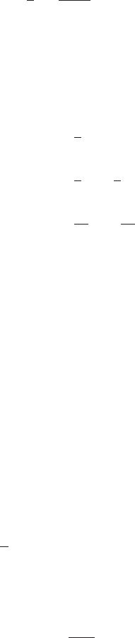
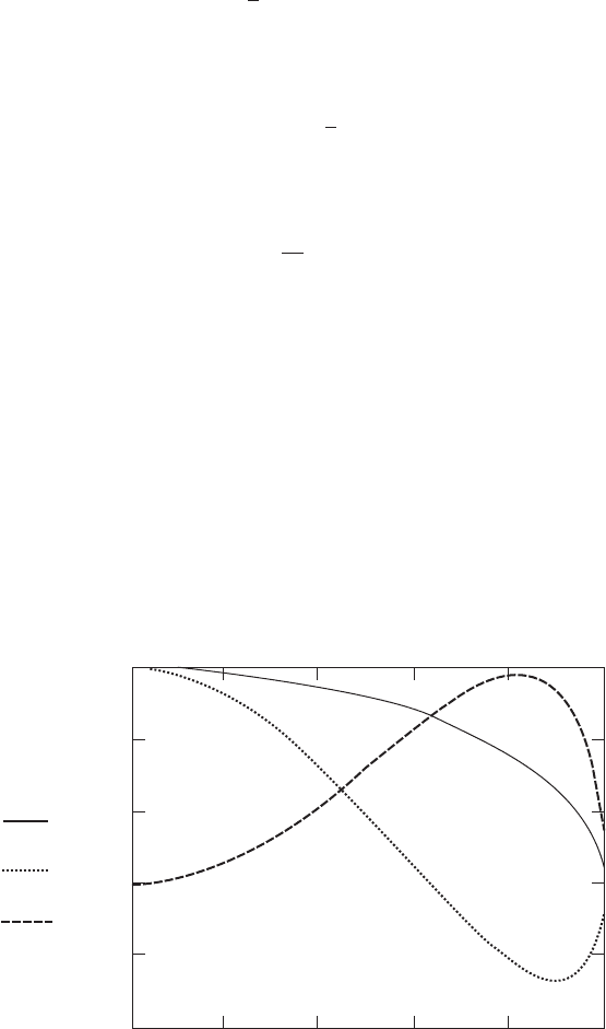
The three distributions are shown in Figure 3.71.

As most modern wind turbines are designed to achieve as uniform a pressure

distribution as practicable, to maximiz e efﬁciency, the form chosen for the helicop-

ter rotor might need to be modiﬁed. A uniform pressure distribution can be formed

by combining solutions but, because the pressure discontinuity must itself be

discontinuous at the disc edge, it would mean that a great many solutions would be

required. Tip-loss effects would require zero pressure at both the blade tips and at

the hub but for most of the blade span the pressure should be uniform. It should be

pointed out that the blade loading caused by uniform pressure does increase linearly

with radius.

The induced velocity ﬁeld caused by the axisymmetric pressure distribution has

to be obtained from the pressure ﬁeld by integrating Equations (3.145) commencing

far upstream where free-stream conditions are assumed to apply. The upstream

1.5

1.0

0.5

0.0

-0.5

-1.0

0 0.2 0.4 0.6 0.8 1

(µ)

Figure 3.71 Radial Pressure Distributions of the First Two Solutions and their Combination

to Satisfy the Requirements at the Rotor Axis

THE METHOD OF ACCELERATION POTENTIAL 131

conditions also depend upon the angle of yaw of the disc. The integration continues

until a point on the disc is reached where the induced velocity is to be determined.

The particular induced velocity component that is most important for determin-

ing the angle of attack on a blade element is normal to the rotor disc, i.e., the axial

induced velocity. Mangler and Squire (1950) calculated the axial induced velocity

distribution as a function of yaw angle by expressing the velocity as a Fourier series

of the azimuth angle ł.

¼ C

( , ª)

k¼1

( , )sin kł

(3:167)

For the pressure distribution of Equation (3.166) the Fourier coefﬁcients are

( , ª) ¼



(1  

)

1=2

(3:168a)

( , ª) ¼

15

256

(9

 4)tan

(3:168b)

( , ª) ¼

45

256



tan



(3:168c)

Higher-order odd terms are zero. There are also even terms which have the general

form

¼ (1)

(k2)=2

k þ v

 1

þ k

 6

 9



 9



1  v

1 þ v



k=2

tan

k=2

where v

¼ 1  

and k is an even integer greater than zero.

The average val ue of the axial induced ﬂow factor is independent of yaw angle

and is given by

¼

where u

is the average axial induced velocity.

Thus, the average value of the axial ﬂow induced ﬂow factor is related to the

thrust coefﬁcient by

¼ 4a

(3:169)

compared with the momentum theory C

¼ 4a

(1  a

) or compared with any of

the expressions developed for yawed conditions (Equations (3.91), (3.106) and

(3.112)).

Because of the assumption that the induced velocity is small compared with the

ﬂow velocity, a

is small compared with 1. Clearly, the acceleration potential

method only appl ies if the value of C

is much less than 1.

132 AERODYNAMICS OF HORIZONTAL-AXIS WIND TURBINES

The once per revolution term in Equation (3.167) will cause an angle of attack

variation and, hence, a lift variation that will cause a yawing moment on the disc.

However, the pressure distribution, being axi-symmetric, cannot cause a yawing

moment. The situation is much the same as for the vortex theory of Coleman,

Feingold and Stempin (1945).

Pitt and Peters (1981) use, or rather, impose Glauert’s assumption (Equation

(3.108)) for the variation of the axial induced ﬂow factor:

a ¼ a

þ a

 sin ł (3:170)

The value of a

is obtained by equating the ﬁrst moment about the yaw axis of

Equation (3.170) with the ﬁrst moment of Equation (3.167) using the Mangler and

Squire velocity distributions of Equations (3.168).

2

 sin ł(a

þ a

 sin ł)2 d dł

2

 sin łC

(, ª)

k¼1

( , ª)sin kł

 d d ł (3:171)

All terms, apart from that co ntaining A

, vanish on integration, giving

15

128

tan

(3:172)

Hence, using Equation (3.169), the axial induced velocity becomes

a ¼ a

1 þ

15

 tan

sin ł



(3:173)

Which, apart from the use of the yaw angle instead of the wake skew angle, has the

same form as Equations (3.108) and (3.118) and so there is some consistency in the

various methods for dealing with yawed ﬂow.

3.11.4 The anti-symmetric pressure distributions

As has been determined in Section 3.10.11, there is a moment about the vertical

diameter of a yawed wind turbine rotor disc, the restoring yaw moment. An axi-

symmetric pressure distr ibution, however, is not capable of producing a yaw

moment and so more terms from the series solution of Equation (3.159) need to be

included.

The only terms in Equation (3.159) which wil l yield a yawing moment are those

for which m ¼ 1 and for which D

6¼ 0. Terms for which m ¼ 1 and C

6¼ 0 will

cause a tilting moment. Recalling that m þ n must be odd to achieve a pressure

discontinuity across the disc the values of n that may be combined with m ¼ 1 must

be even.

THE METHOD OF ACCELERATION POTENTIAL 133

Because of the nature of the Legendre polynomials only one term in the series of

Equation (3.159) will produce a net thrust and only one term will produce a yawing

moment, which is a ﬁrst moment. Similarly only one term will produce a second

moment, and so on.

The unique term in Equation (3.159) which yields a yawing moment is that for

which m ¼ 1, n ¼ 2 and C

6¼ 0, therefore

(v) ¼ 3v

ﬃﬃﬃﬃﬃﬃﬃﬃﬃﬃﬃﬃﬃ

1  v

¼ 3

ﬃﬃﬃﬃﬃﬃﬃﬃﬃﬃﬃﬃﬃﬃ

1  

(3:174)

and

(i) ¼ 3i

ﬃﬃﬃﬃﬃﬃﬃﬃﬃﬃﬃﬃﬃ

1 þ 

tan

1



 3i

ﬃﬃﬃﬃﬃﬃﬃﬃﬃﬃﬃﬃﬃ

1 þ 

ﬃﬃﬃﬃﬃﬃﬃﬃﬃﬃﬃﬃﬃ

1 þ 

,(3:175)

(i0) ¼2i (3:175a)

A zero pressure gradient at the rotor axis is not appropriate in this case because the

pressure distribution is anti-symmetric about the yaw axis, therefore,

p( , ł) ¼ P

( )Q

(i0)D

sin ł ¼6iD



ﬃﬃﬃﬃﬃﬃﬃﬃﬃﬃﬃﬃﬃﬃ

1  

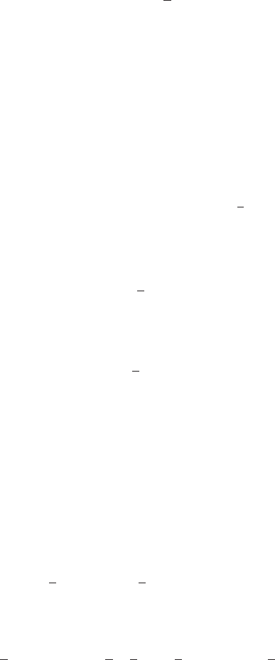
sin ł (3:176)

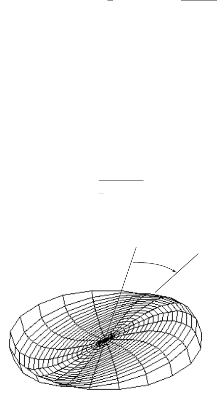
The pressure distribution is shown in Figure 3.72.

The yawing moment coefﬁcient is deﬁned by

R

(3:177)

As before, if the pressure in Equation (3.176) is non-dimensionalized by the free-

stream dynamic pressure (1=2)rU

, then

Figure 3.72 The Form of the Pressure Distribution which Yields a Yawing Moment

134

AERODYNAMICS OF HORIZONTAL-AXIS WIND TURBINES

Burton T. (et. al.) Wind energy Handbook

Подождите немного. Документ загружается.