Brizard A. An Introduction to Lagrangian Mechanics

Подождите немного. Документ загружается.

6.2. ACCELERATIONS IN ROTATING FRAMES 105

Figure 6.2: General rotating frame

since the second term in Eq. (6.4) vanishes for A = ω; the time derivative of ω is, therefore,

the same in both frames of reference and is denoted

ω in what follows.

6.2 Accelerations in Rotating Frames

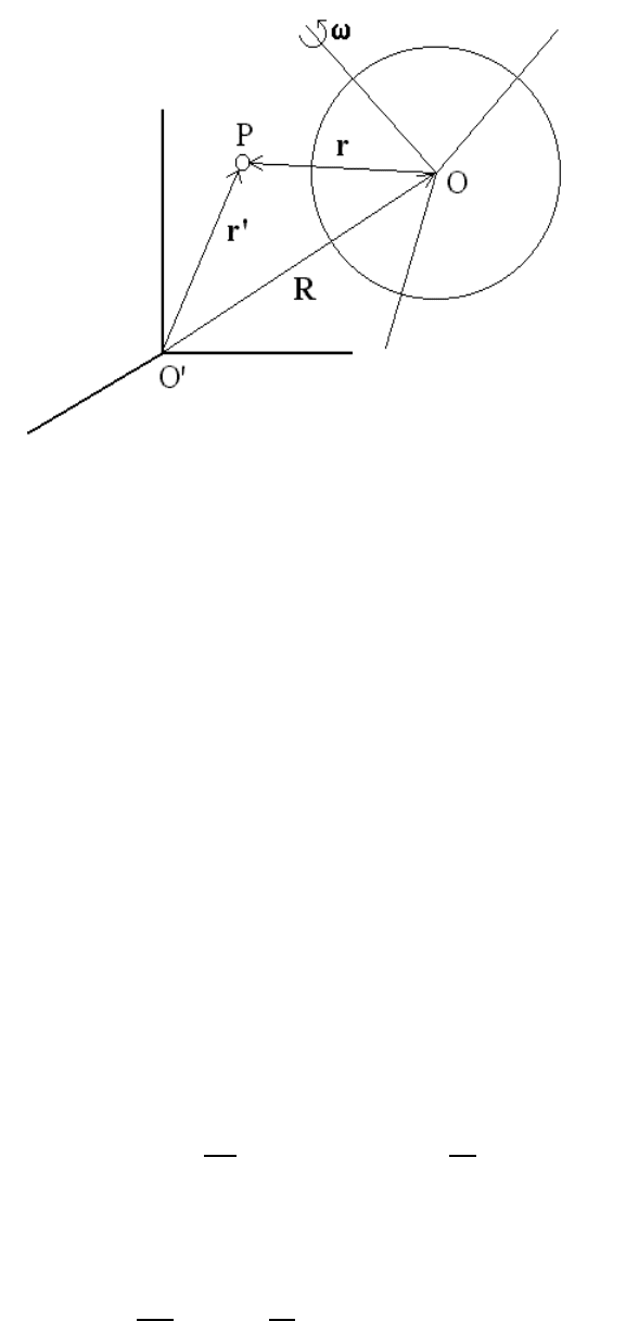
We now consider the general case of a rotating frame and ﬁxed frame being related by

translation and rotation. In Figure ??, the position of a point P according to the ﬁxed

frame of reference is labeled r

, while the position of the same point according to the

rotating frame of reference is labeled r, and

= R + r, (6.5)

where R denotes the position of the origin of the rotating frame according to the ﬁxed

frame. Since the velocity of the point P involves the rate of change of position, we must

now be careful in deﬁning which time-derivative operator, (d/dt)

or (d/dt)

, is used.

The velocities of point P as observed in the ﬁxed and rotating frames are deﬁned as

and v

, (6.6)

resp ectively. Using Eq. (6.4), the relation between the ﬁxed-frame and rotating-frame

velocities is expressed as

= V + v

+ ω × r, (6.7)

106 CHAPTER 6. MOTION IN A NON-INERTIAL FRAME

where V =(dR/dt)

denotes the translation velocity of the rotating-frame origin (as

observed in the ﬁxed frame).

Using Eq. (6.7), we are now in a position to evaluate expressions for the acceleration of

point P as observed in the ﬁxed and rotating frames of reference

and a

, (6.8)

resp ectively. Hence, using Eq. (6.7), we ﬁnd

dω

× r + ω ×

= A +(a

+ ω × v

ω × r + ω × (v

+ ω × r) ,

= A + a

+2ω × v

ω × r + ω × (ω × r) , (6.9)

where A =(dV/dt)

denotes the translational acceleration of the rotating-frame origin

(as observed in the ﬁxed frame of reference). We can now write an expression for the

acceleration of point P as observed in the rotating frame as

= a

− A − ω × (ω × r) − 2 ω × v

−

ω × r, (6.10)

which represents the sum of the net inertial acceleration (a

− A), the centrifugal accel-

eration −ω × (ω × r) and the Coriolis acceleration −2ω × v

(see Figures 6.3) and an

angular acceleration term −

ω × r which depends explicitly on the time dependence of the

rotation angular velocity ω .

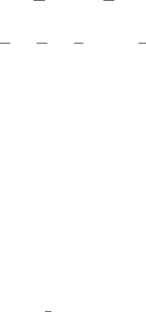
The centrifugal acceleration (which is directed outwardly from the rotation axis) rep-

resents a familiar non-inertial eﬀect in physics. A less familiar non-inertial eﬀect is the

Coriolis acceleration discovered in 1831 by Gaspard-Gustave Coriolis (1792-1843). Figure

6.3 shows that an object falling inwardly also experiences an eastward acceleration.

6.3 Lagrangian Formulation of Non-Inertial Motion

We can recover the expression (6.10) for the acceleration in a rotating (non-inertial) frame

from a Lagrangian formulation as follows. The Lagrangian for a particle of mass m moving

in a non-inertial rotating frame (with its origin coinciding with the ﬁxed-frame origin) in

the presence of the p otential U( r) is expressed as

L(r,

r)=

r + ω × r|

− U(r), (6.11)

6.3. LAGRANGIAN FORMULATION OF NON-INERTIAL MOTION 107

Figure 6.3: Centrifugal and Coriolis accelerations

where ω is the angular velocity vector and we use the formula

r + ω × r|

= |

+2ω · (r ×

r)+

− ( ω · r)

Using the Lagrangian (6.11), we now derive the general Euler-Lagrange equation for r.

First, we derive an expression for the canonical momentum

p =

∂L

∂

= m (

r + ω × r) , (6.12)

and

∂L

∂

= m (

r +

ω × r + ω ×

r) .

Next, we derive the partial derivative

∂L

∂r

= −∇U(r) − m [ ω ×

r + ω × (ω × r)],

so that the Euler-Lagrange equations are

r = −∇U(r) − m [

ω × r +2ω ×

r + ω × (ω × r)]. (6.13)

Here, the p otential energy term generates the ﬁxed-frame acceleration, −∇U = m a

, and

thus the Euler-Lagrange equation (6.13) yields Eq. (6.10).

108 CHAPTER 6. MOTION IN A NON-INERTIAL FRAME

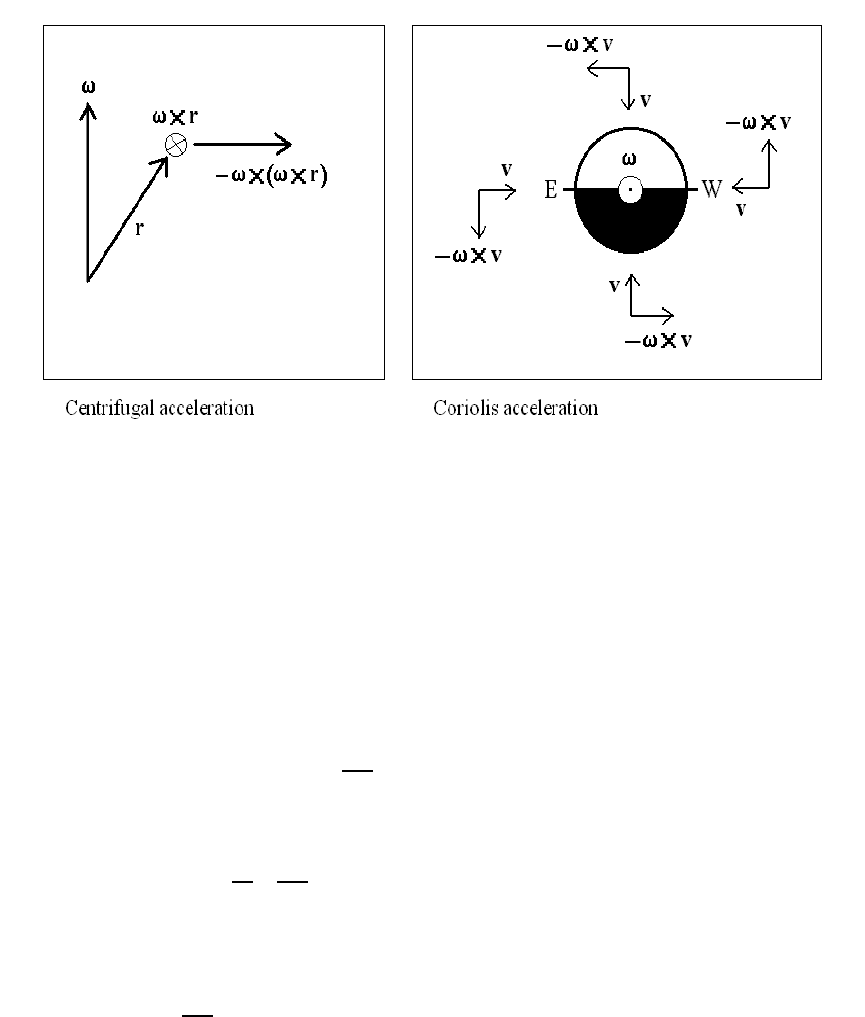
Figure 6.4: Earth frame

6.4 Motion Relative to Earth

We can now apply these non-inertial expressions to the important case of the ﬁxed frame of

reference having its origin at the center of Earth (p oint O

in Figure 6.4) and the rotating

frame of reference having its origin at latitude λ and longitude ψ (point O in Figure 6.4).

We note that the rotation of the Earth is now represented as

ψ = ω and that

ω =0.

We arrange the (x, y, z) axis of the rotating frame so that the z-axis is a continuation

of the p osition vector R of the rotating-frame origin, i.e., R = R

z in the rotating frame

(where R = 6378 km is the radius of a spherical Earth). When expressed in terms of the

ﬁxed-frame latitude angle λ and the azimuthal angle ψ, the unit vector

z is

z = cos λ (cos ψ

+ sin ψ

) + sin λ

i.e.,

z points upward. Likewise, we choose the x-axis to be tangent to a great circle passing

through the North and South p oles, so that

x = sin λ (cos ψ

+ sin ψ

) − cos λ

i.e.,

x points southward. Lastly, the y-axis is chosen such that

y =

z ×

x = − sin ψ

+ cos ψ

i.e.,

y points eastward.

We now consider the acceleration of a point P as observed in the rotating frame O by

writing Eq. (6.10) as

= g

−

− ω × (ω × r) − 2 ω ×

. (6.14)

6.4. MOTION RELATIVE TO EARTH 109

The ﬁrst term represents the pure gravitational acceleration due to the graviational pull of

the Earth on point P (as observed in the ﬁxed frame located at Earth’s center)

= −

where r

= R + r is the position of point P in the ﬁxed frame and r is the location of

P in the rotating frame. When expressed in terms of rotating-frame spherical coordinates

(r, θ, ϕ):

r = r [ sin θ (cos ϕ

x + sin ϕ

y)+cosθ

z ] ,

the ﬁxed-frame position r

is written as

=(R + r cos θ)

z + r sin θ (cos ϕ

x + sin ϕ

y) ,

and thus



+2Rr cos θ + r



3/2

The pure gravitational acceleration is, therefore, expressed in the rotating frame of the

Earth as

= − g

(1 +  cos θ)

z +  sin θ (cos ϕ

x + sin ϕ

(1+2 cos θ + 

)

3/2

, (6.15)

where g

= GM/R

=9.789 m/s

and  = r/R  1.

The angular velocity in the ﬁxed frame is ω = ω

, where

ω =

2π rad

24 × 3600 sec

=7.27 × 10

−5

rad/s

is the rotation speed of Earth about its axis. In the rotating frame, we ﬁnd

ω = ω (sin λ

z − cos λ

x) . (6.16)

Because the position vector R rotates with the origin of the rotating frame, its time deriva-

tives yield

= ω × R =(ωR cos λ)

= ω ×

= ω × (ω × R)=− ω

R cos λ (cos λ

z + sin λ

x) ,

and thus the centrifugal acceleration due to R is

= − ω × (ω × R )=αg

cos λ (cos λ

z + sin λ

x) , (6.17)

where ω

R =0.0337 m/s

can be expressed in terms of the pure gravitational acceleration

as ω

R = αg

, where α =3.4 × 10

−3

. We now deﬁne the physical gravitational

acceleration as

g = g

− ω × [ ω × (R + r)]

= g

−



1 − α cos



z +(α cos λ sin λ)

, (6.18)

110 CHAPTER 6. MOTION IN A NON-INERTIAL FRAME

where terms of order  have b een neglected. For example, a plumb line experiences a small

angular deviation δ(λ) (southward) from the true vertical given as

tan δ(λ)=

α sin 2λ

(2 − α)+α cos 2λ

This function exhibits a maximum at a latitude

λ deﬁned as cos 2λ = −α/(2 −α), so that

tan

δ =

α sin 2λ

(2 − α)+α cos 2λ

√

1 − α

' 1.7 × 10

−3

δ ' 5.86 arcmin at λ '





rad = 45.05

We now return to Eq. (6.14), which is written to lowest order in  and α as

= − g

z − 2 ω ×

, (6.19)

where

ω ×

= ω [(˙x sin λ +˙z cos λ)

y − ˙y (sin λ

x + cos λ

z)].

Thus, we ﬁnd the three components of Eq. (6.19) written explicitly as

¨x =2ω sin λ ˙y

¨y = − 2 ω (sin λ ˙x + cos λ ˙z)

¨z = − g +2ω cos λ ˙y











. (6.20)

A ﬁrst integration of Eq. (6.20) yields

˙x =2ω sin λy + C

˙y = − 2 ω (sin λx + cos λz)+C

˙z = − gt +2ω cos λy + C











, (6.21)

where (C

) are constants deﬁned from initial conditions (x

) and ( ˙x

, ˙y

, ˙z

=˙x

− 2 ω sin λy

=˙y

+2ω (sin λx

+ cos λz

)

=˙z

− 2 ω cos λy











. (6.22)

A second integration of Eq. (6.21) yields

x(t)=x

+ C

t +2ω sin λ

y dt,

y(t)=y

+ C

t − 2 ω sin λ

xdt − 2 ω cos λ

z dt,

z(t)=z

+ C

t −

+2ω cos λ

y dt,

6.4. MOTION RELATIVE TO EARTH 111

which can also be rewritten as

x(t)=x

+ C

t + δx(t)

y(t)=y

+ C

t + δy(t)

z(t)=z

+ C

t −

+ δz(t)











, (6.23)

where the Coriolis drifts are

δx(t)=2ω sin λ



t +

δy dt



(6.24)

δy(t)=− 2 ω sin λ



t +

δxdt



− 2 ω cos λ



t +

−

δz dt



(6.25)

δz(t)=2ω cos λ



t +

δy dt



. (6.26)

Note that each Coriolis drift can be expressed as an inﬁnite series in powers of ω and that

all Coriolis eﬀects vanish when ω =0.

6.4.1 Free-Fall Problem Revisited

As an example of the importance of Coriolis eﬀects in describing motion relative to Earth,

we consider the simple free-fall problem, where

)=(0, 0,h) and ( ˙x

, ˙y

, ˙z

)=(0, 0, 0),

so that the constants (6.22) are

=0=C

and C

=2ωh cos λ.

Substituting these constants into Eqs. (6.23) and keeping only terms up to ﬁrst order in ω,

we ﬁnd

x(t)=0, (6.27)

y(t)=

ω cos λ, (6.28)

z(t)=h −

. (6.29)

Hence, a free-falling object starting from rest touches the ground z(T ) = 0 after a time

T =

2h/g after which time the object has drifted eastward by a distance of

y(T )=

ω cos λ =

ω cos λ

At a height of 100 m and latitude 45

, we ﬁnd an eastward drift of 1.55 cm.

112 CHAPTER 6. MOTION IN A NON-INERTIAL FRAME

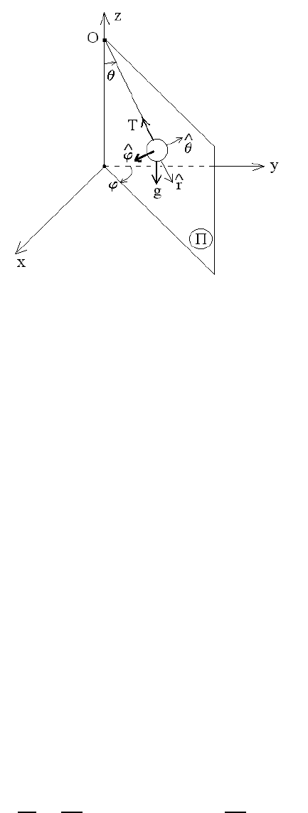
Figure 6.5: Foucault pendulum

6.4.2 Foucault Pendulum

In 1851, Jean Bernard L´eon Foucault (1819-1868) was able to demonstrate the role played

by Coriolis eﬀects in his investigations of the motion of a pendulum (of length ` and mass

m) in the rotating frame of the Earth. His analysis showed that, because of the Coriolis

acceleration associated with the rotation of the Earth, the motion of the pendulum exhibits

a precession motion whose period depends on the latitude at which the pendulum is located.

The equation of motion for the pendulum is given as

r = a

− 2 ω ×

r, (6.30)

where a

= g+T/m is the net ﬁxed-frame acceleration of the pendulum expressed in terms

of the gravitational acceleration g and the string tension T (see Figure 6.5). Note that

the vectors g and T span a plane Π in which the pendulum moves in the absence of the

Coriolis acceleration − 2ω ×

r. Using spherical coordinates (r, θ, ϕ) in the rotating frame

and placing the origin O of the pendulum system at its pivot point (see Figure 6.5), the

position of the pendulum bob is

r = ` [ sin θ (sin ϕ

x + cos ϕ

y) − cos θ

z ]=`

r(θ, ϕ). (6.31)

From this deﬁnition, we construct the unit vectors

θ and

ϕ as

θ =

∂

∂θ

∂

∂ϕ

= sin θ

ϕ, and

∂

∂ϕ

= cos θ

ϕ. (6.32)

Note that, whereas the unit vectors

r and

θ lie on the plane Π, the unit vector

ϕ is

perpendicular to it and, thus, the equation of motion of the pendulum perpendicular to the

6.4. MOTION RELATIVE TO EARTH 113

plane Π is

r ·

ϕ = − 2(ω ×

r) ·

ϕ. (6.33)

The pendulum velocity is obtained from Eq. (6.31) as

r = `



θ +˙ϕ sin θ



, (6.34)

so that the azimuthal component of the Coriolis acceleration is

− 2(ω ×

r) ·

ϕ =2`ω

θ (sin λ cos θ + cos λ sin θ sin ϕ) .

If the length ` of the pendulum is large, the angular deviation θ of the pendulum can be

small enough that sin θ  1 and cos θ ' 1 and, thus, the azimuthal component of the

Coriolis acceleration is approximately

− 2(ω ×

r) ·

ϕ ' 2 ` (ω sin λ)

θ. (6.35)

Next, the azimuthal component of the p endulum acceleration is

r ·

ϕ = `



¨ϕ sin θ +2

θ ˙ϕ cos θ



which for small angular deviations yields

r ·

ϕ ' 2 ` (˙ϕ)

θ. (6.36)

By combining these expressions into Eq. (6.33), we obtain an expression for the precession

angular frequency of the Foucault pendulum

˙ϕ = ω sin λ (6.37)

as a function of latitude λ. As expected, the precession motion is clockwise in the Northern

Hemisphere and reaches a maximum at the North Pole (λ =90

). Note that the precession

period of the Foucault pendulum is (1 day/ sin λ) so that the period is 1.41 days at a

latitude of 45

or 2 days at a latitude of 30

The more traditional approach to describing the precession motion of the Foucault pen-

dulum makes use of Cartesian coordinates (x, y, z). The motion of the Foucault pendulum

in the ( x, y)-plane is described in terms of Eqs. (6.30) as

¨x + ω

x =2ω sin λ ˙y

¨y + ω

y = −2 ω sin λ ˙x

)

, (6.38)

where ω

= T/m` ' g/` and ˙z ' 0if` is very large. Figure 6.6 shows the numerical

solution of Eqs. (6.38) for the Foucault pendulum starting from rest at (x

)=(0, 1)

with 2 (ω/ω

) sin λ =0.05 at λ =45

. The left ﬁgure in Figure 6.6 shows the short time

behavior (note the diﬀerent x and y scales) while the right ﬁgure in Figure 6.6 shows the

complete Foucault precession. Figure 6.7 shows that, over a ﬁnite period of time, the

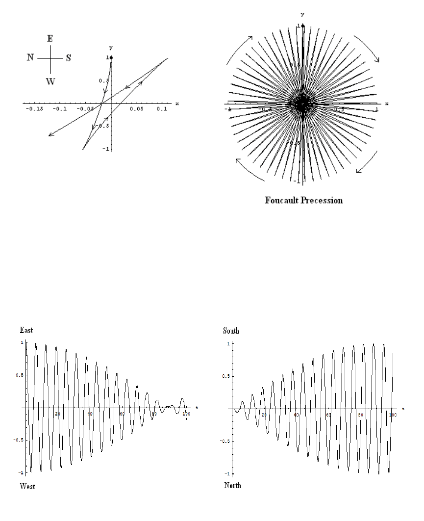
114 CHAPTER 6. MOTION IN A NON-INERTIAL FRAME

Figure 6.6: Solution of the Foucault pendulum

Figure 6.7: Projection of Foucault pendulum