Brewster H.D. Fluid Mechanics
Подождите немного. Документ загружается.

182
Hydrostatics and Aerostatics
it can be inferred that a large part
of
the bubble forms
at
an
almost constant
vertex radius
and
it
is
an
important property for larger nozzle radii.
For
smaller nozzle radii, stronger/larger changes
of
the vertex raoius are
to
be
expected during the formation
of
the gas bubbles.
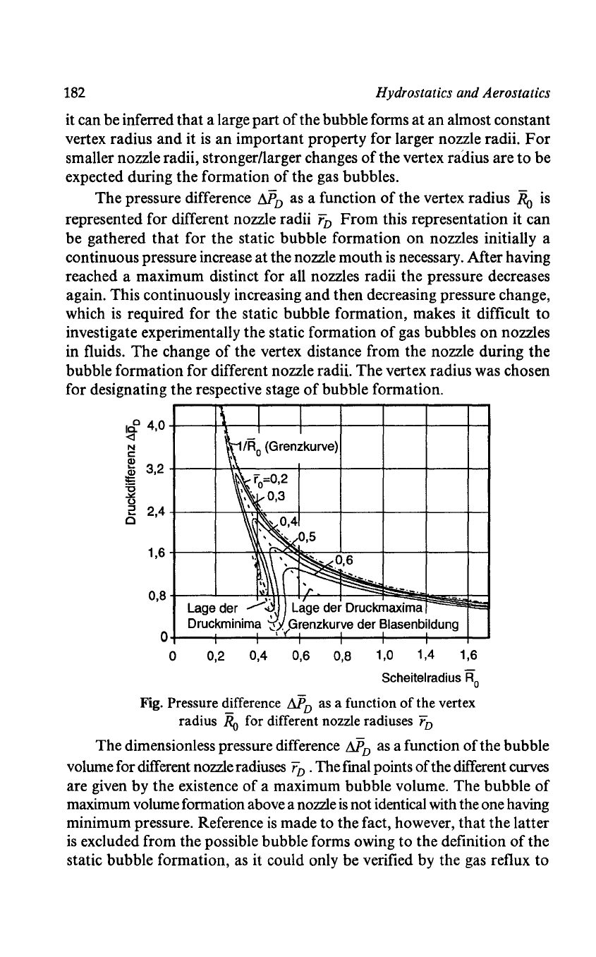
The pressure difference
MD
as a function
of
the vertex radius
Ro
is
represented for different nozzle radii
rD
From
this representation it can
be gathered
that
for the static bubble formation
on
nozzles initially a
continuous pressure increase
at
the nozzle mouth
is
necessary. After having
reached a maximum distinct for all nozzles radii the pressure decreases
again. This continuously increasing and then decreasing pressure change,
which
is
required for the static bubble formation, makes it difficult to
investigate experimentally the static formation
of
gas bubbles
on
nozzles
in fluids. The change
of
the vertex distance from the nozzle during the
bubble formation for different nozzle radii. The vertex radius was chosen
for designating the respective stage
of
bubble formation.
I~
4,0+---~~--~--~---+----+---~--~~
<l
N
c:
~
~
3,2
~
c
2,4
+---~--*""'~---+---_+----+---~--~~
1,6
+---_+------II~~~:--____!__::__--+---_+--__If___I
0,8t-=~~,.
~~E~~-'-~~~
Lage der
....-.,
Lage der Druckmaxima
Druckminima
~
. Grenzkurve der Blasenbildung
O+---~---+~'~~--~--~----~--+-~
o 0,2 0,4 0,6 0,8 1,0 1,4 1,6
Scheitelradius
Ro
Fig. Pressure difference
MD
as a function
of
the vertex
radius
Ro
for different nozzle radiuses
rD
The dimensionless pressure difference
MD
as a function
of
the bubble
volume for different nozzle radiuses
rj; . The [mal points
of
the different curves
are given by the existence
of
a maximum bubble volume. The bubble
of
maximum volume formation above a nozzle
is
not identical with the one having
minimum pressure. Reference
is
made to the fact, however,
that
the latter
is
excluded from the possible bubble forms owing to the definition
of
the
static bubble formation,
as it could only be verified by the gas reflux to
Hydrostatics and Aerostatics
183
the nozzles.
For
general comprehension
of
the problem
of
static bubble
formation, two further facts can be referred to:
•
For
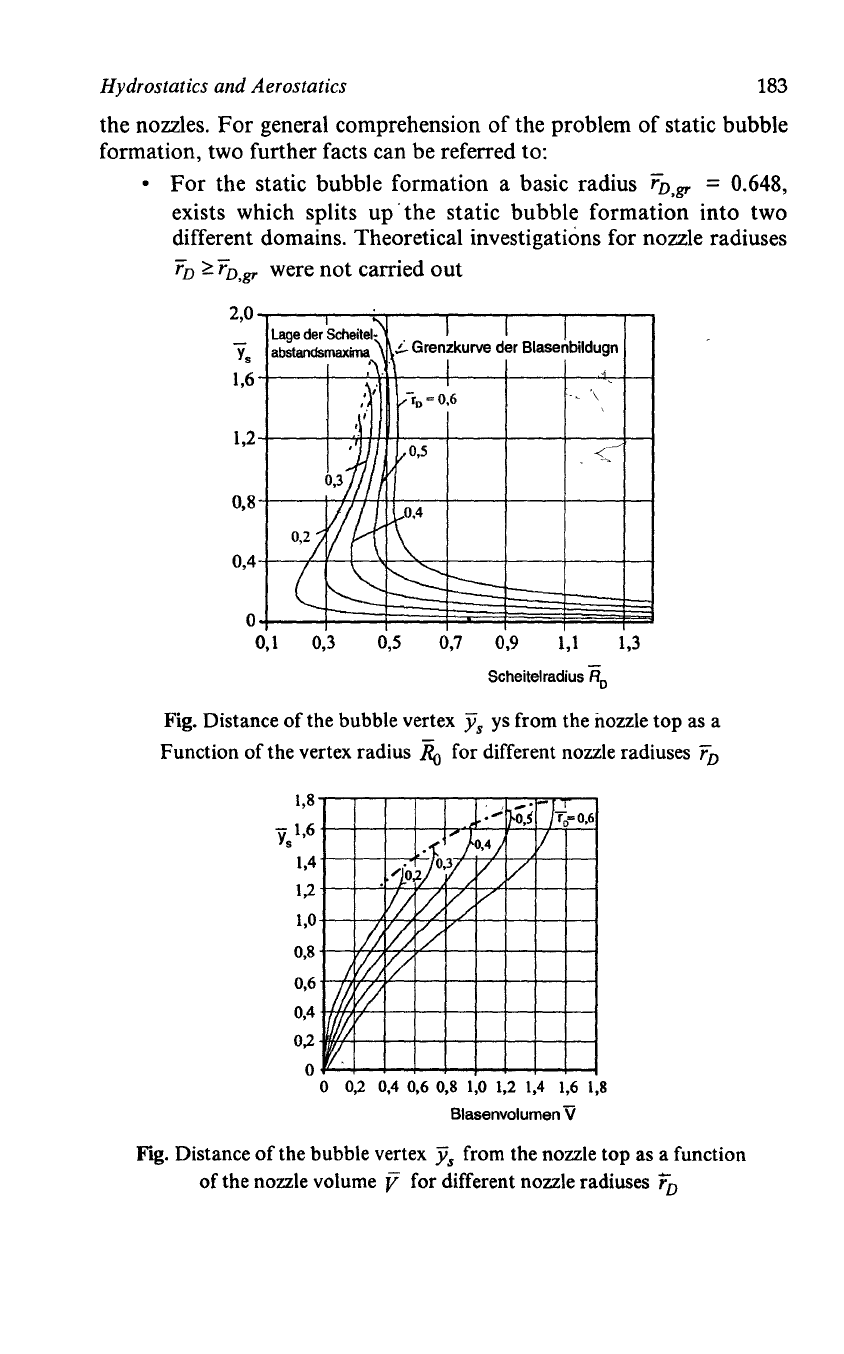
the static bubble formation a basic radius rD,gr = 0.648,
exists which splits
up'
the static bubble formation into two
different domains. Theoretical investigations for nozzle radiuses
rD
~
rD,gr were not carried out
2,0
y.
1,6
Lage
der
IScheit~l\
abstandsmaxm;\ .
, ,
,
I{
i-
Gren~kurve
d~r
Blase~bildUgn
. I
I
V
f
D
cO
,6
-,
\
1,2
,I)
!to.S
<;.~
O.l!!/,
~
\-,0,4
O'Z;
\
C
~
~
~
I--
0,8
0,4
o
0,1
0,3
0,5
0,7
0,9
1,1
1,3
Scheitelradius
Ro
Fig. Distance
of
the bubble vertex
}is
ys from the nozzle top as a
Function
of
the vertex radius
Ro
for different nozzle radiuses
rD
1,8
'1.
1
,6
1,4
1,2
1,0
0,8
0,6
0,4
0,2
o
j'
....
(0$
-
)r;,=0.6
.
.,:l
....
}?4j
V
.
/Lo~JO'Y
V
/
VI
~
V/
V
/;
::0
~
/~
'i'
III
'/j
WI/;
r.
o
0,2
0,4
0,6 0,8
1,0
1,2
1,4
1,6
1,8
Blasenvolumen V
Fig. Distance
of
the bubble vertex
}is
from the nozzle top as a function
of
the nozzle volume V for different nozzle radiuses
'D
184 Hydrostatics and Aerostatics
here, as they are not
of
importance for the introduction
of
the results
intended here for better comprehension
of
the bubble formation.
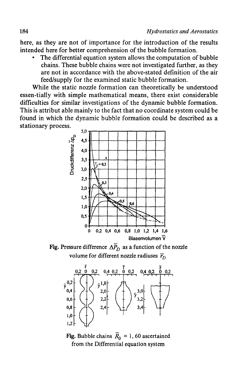
• The differential equation system allows the computation
of
bubble
chains. These bubble chains were not investigated further,
as
they
are not in accordance with the above-stated definition
of
the air
feed/supply for the examined static bubble formation.
While the static nozzle formation can theoretically be understood
essen-tially with simple mathematical means, there exist considerable
difficulties for similar investigations
of
the dynamic bubble formation.
This
is
attribut able mainly to the fact that no coordinate system could be
found in which the dynamic bubble formation could be described as a
stationary process.
5,0
c
Co
4,5
1<1
N
c
4,0
~
&
3,5
'6
-'"
0
~
3,0
~
0
2,5
2,0
1,5
1,0
0,5
•
_\3>=0,2
-'\
A
~,3
.,
~O,4
/
fI
~~
M
(I
~~
~
~
........
~-
........
o
o
0,2 0,4 0,6 0,8 1,0
1,2
1,4 1,6
Blasenvolumen
Ii
Fig. Pressure difference
MD
as a function
of
the nozzle
volume for different nozzle radiuses
rD
r r r
o 0,2 0,4 0,2 0 0,2 0,4 0 0
0,2
_0,2
YI$I
y
3
,of
y
0,4
2,0
0,6
2,2
3,2
0,8 2,4 3,4
1,0
1,2
Fig. Bubble chains
Ro
=
1,60
ascertained
from the Differential equation system
Hydrostatics and Aerostatics
185
Moreover,
for
the dynamic
bubble
formation
the
pressure
on
an
element
of
the interface boundary surface
is
dependent
on
the fluid motions
during bubble formation
and
thus
is
computable only by solving
the
non-
stationary Navier-Stokes equation. This, however,
is
solvable only with
difficulty
and
big computing e orts.
AEROSTATICS
Pressure
in
the
Atmosphere
Aerostatics differs from hydrostatics in
that
for designating
the
fluid,
the partial differential equations for fluids
at
rest derived from the Navier-
Stokes equations are applied along with the equation
of
state
for
an ideal
gas
rather
than
for
an
ideal fluid p = const.
P
=RT
~
P
Thus the valid partial differential equations in aerostatics read:
ap
A P A
ax]
=pg]
=
RT
g
]
or
written
out
for j =
1,
2,
3:
ap
P A
ap
P A
ap
P A
aXl
=
RT
gl
'=
Rx2
=
RT
g2
'
aX3
=
RT
g3
·
This theorem
of
partial differential equations can now be employed for
the computation
of
the pressure distribution in such fluids whose state designa-
tion
is
possible with a precision
that
is
sufficient for the considerations to be
made due
to
the ideal gas equation.
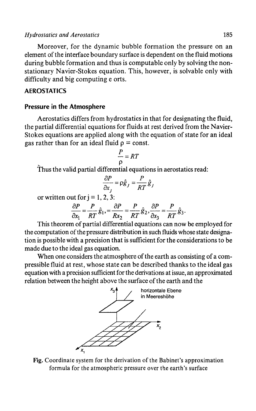
When one considers the atmosphere
of
the earth
as
consisting
of
a com-
pressible fluid
at
rest, whose state can be described thanks
to
the ideal gas
equation with a precision sufficient for the derivations at
issue,
an approximated
relation between the height above the surface
of
the earth and the
horizontale Ebene
in Meereshohe
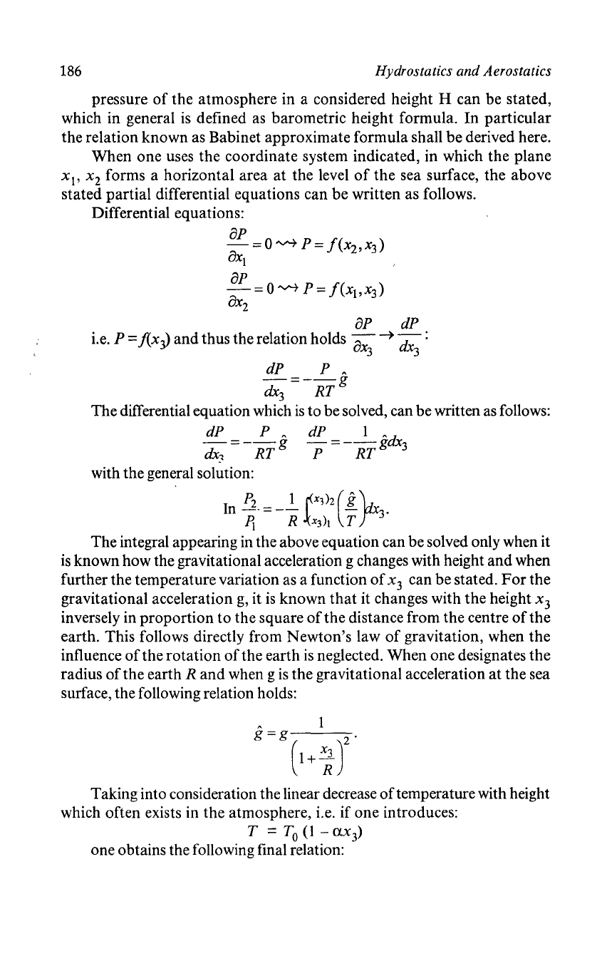
Fig. Coordinate system for the derivation
of
the Babinet's approximation
formula for the atmospheric pressure over the earth's surface
186
Hydrostatics and Aerostatics
pressure
of
the
atmosphere in a considered height H can be stated,
which in general
is
defined
as
barometric height formula. In particular
the relation known as Babinet approximate formula shall be derived here.
When one uses the coordinate system indicated, in which the plane
xl'
x
2
forms a horizontal area at the level
of
the
sea surface, the above
stated partial differential equations can
be
written as follows.
Differential equations:
8P
-=O~
P=!(x2,x3)
8xl
8P
-=O~
P=!(Xl,x3)
8x2
8P dP
i.e. P =
!(x~
and
thus the relation holds
-a
~
-d
:
X3
X3
dP P
~
-=--g
dx
3
RT
The differential equation which
is
to be solved, can be written
as
follows:
dP =
_J:..-.
g dP =
__
1_
gdx
3
dx
1
RT
P
RT
with the general solution:
In
~.
= -
~
t:3~2(:
yX3.
The integral appearing in the above equation can be solved only when it
is
known how the gravitational acceleration g changes with height
and
when
further the temperature variation as a function
of
x3 can be stated.
For
the
gravitational acceleration
g,
it
is
known
that
it changes with
the
height x3
inversely in proportion to the square
of
the distance from the centre
of
the
earth. This follows directly from Newton's law
of
gravitation, when the
influence
of
the rotation
of
the earth
is
neglected. When one designates
the
radius
of
the earth R
and
when g
is
the gravitational acceleration
at
the sea
surface, the following relation holds:
~
1
g
=g(
)2.
1 +
x3
R
Taking into consideration the linear decrease
of
temperature with height
which often exists in the atmosphere, i.e. if one introduces:
T =
To
(l
-
ax
3)
one obtains the following final relation:
Hydrostatics and Aerostatics
187
H
In
PH
=_-L
I
dx
3
.
Po
RTo
0 (1-<x'x
3
)(1+
~
r
When one now imposes restrictions concerning the height above which
the
above-indicated integration
is
to
take
place
and
when
one
chooses
them
such
that
the
following relations hold:
x3
<X.X3<
1-<
1
R
one can obtain by exponential-series development:
PH
g
HI
(
2x3
)
In
--=--
(l+<x'x3
+
...
)
1--+
...
dX3
Po
RTo
0 R
or
the approximate formula by neglecting the terms
of
higher order:
In
PH
=--L1[1+(l-~)X3l-1-3'
.
Po
RTo
0 R J
By
solving this equation the following fmal relation results for the pressure
distribution in the lower atmosphere:
PH
~poexpH~[l+M
(X-
~)H]}
This preSsure relation describes with good precision the standard pressure
distribution existing in the atmosphere.
The approximate formulae stated by Babinet for the pressure distribution
in the atmosphere can be derived from
the
general differential equation
dP
_ g
----
dx
3
P 'RT
by introducing the following hypotheses:
PH+P
o
P = = const g = g
=const
2
To+TH
T = =const.
2
When
one
introduces these simplifications/reductions,
the
following
solution for the differential equation results:
2 H g
---(PH
-P
o
)=-
f-
dx
3
PH
+P
o
0 RT
or
resolved:
PH
-Po
==
gH
PH
+
Po
R(To
+ T
H
)
188
Hydrostatics
and
Aerostatics
H=-
RTO(l+
TH)(P
H
-Po).
g
To
PH
+P
o
When one rearranges this equation according to
Po
it results:
RTO(I+
TH
)-H
PH
~Po
~TO(I+;:
)+H
g
To
The two relations in comparison to the standard pressure distribution
in the atmosphere.
Rotating Containers
As a further example for the employment
of
the aerostatic basic
equations.
By
a single pressure measurement in the upper centre point
of
the cylinder ceiling surface and by employment
of
the partial differential
equation
of
aerostatics the entire pressure load on the circumferential
surface
of
a rotating cylinder filled with a compressible medium shall be
defined.
25.-----------------------------~
iii
100
.0
E..
~
75
--
o..l:
..l<:
50
u
::l
o
25
--
Normdruck
- - -
Gleichung (6.98)
_.-
..
Gleichung
(6.104)
-.-
°0~--~20~0~--~4+.00~--~6~onO----~8OO~--~1~000
H6he H
/10
[m]
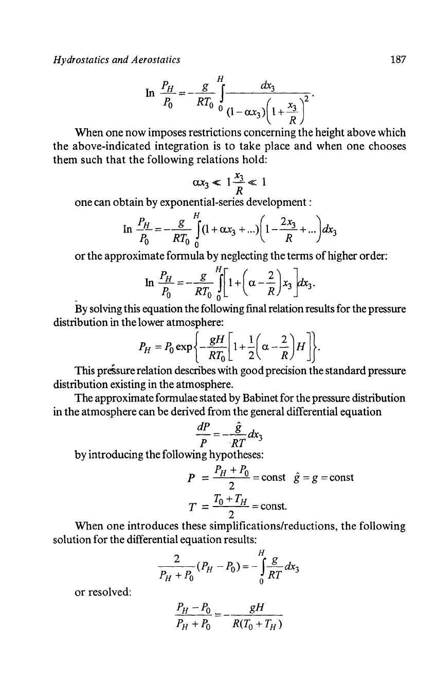
Fig. Standard pressure distribution in the atmosphere and
distributions computed on the basis
of
approximate formulas
Contrary to the example treated here the cylinder shall experience a
pure rotational motion only, so that the partial differential equations
of
aerostatics can be written for T = const as follows:
oP
P
00
2
2
-=-roo
2
~InP=--r
+F(<p,Z),
&
RT
2RT
loP
.--
=0
~
P =
F(r
z)
r
o<p
, ,
Hydrostatics and Aerostatics
8P
P g
8z
=-
RTg~InP=-
RTz+F(r,cp).
By
comparing the solutions one obtains:
2
InP=C+~r2
-~z.
2RT
RT
189
The
pressure
Po,
measured
at
the
coordinate
origin permits
the
definition
of
the
integration constant
Cas:
C
=lnP
o
'
From
this P
is
computed:
P =
poexp{~r2
-~z}
2RT
RT
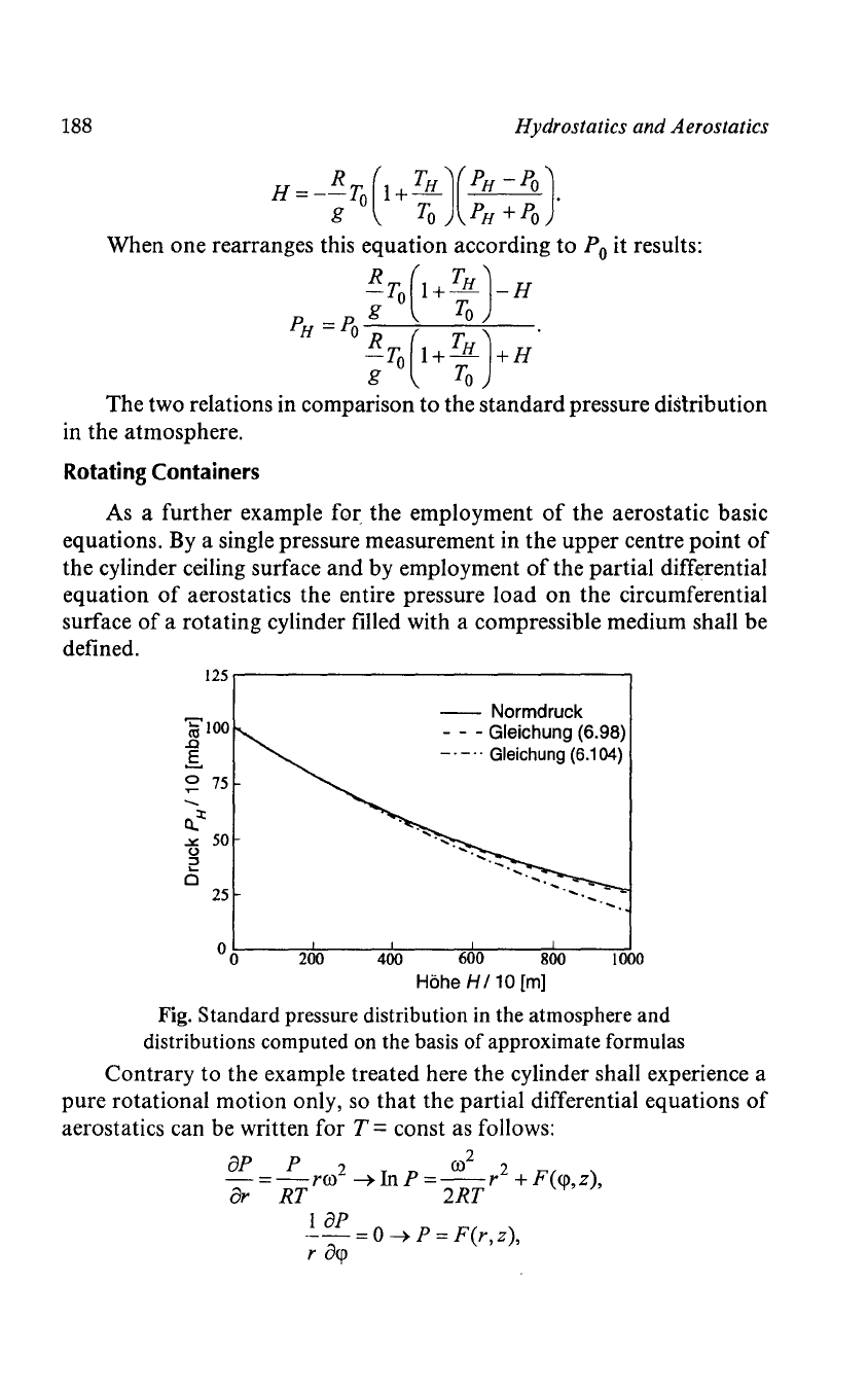
Along the floor space z = -L the pressure distribution
is
computed
as:
PL;
Die Druckverteilung in
rotierenden
Behaltern mit
kompressilblen Fluiden
kann sehr komplex werden
Fig.
Rotating
cylinder
with
a compressible Medium
P(r z = - L) =
Po
exp{~r2
+
gL}.
,
2RT
RT
Along the vertical circumferential surface r = R holds:
P(r
= R,
z)
=
Po
exp{~r2
-~z}.
2RT
RT
Aerostatic Buoyancy
When employing aerostatic laws, mistakes are often made by using
relations whose validity strictly speaking
is
only in hydrostatics. As an example
is
cited at this place the buoyancy
of
bodies which
is
computed according
to figure as the difference
of
the pressure forces
on
the lower
and
upper
sides
of
a immersed body.
The
basic equations for these computations.
190
Hydrostatics and Aerostatics
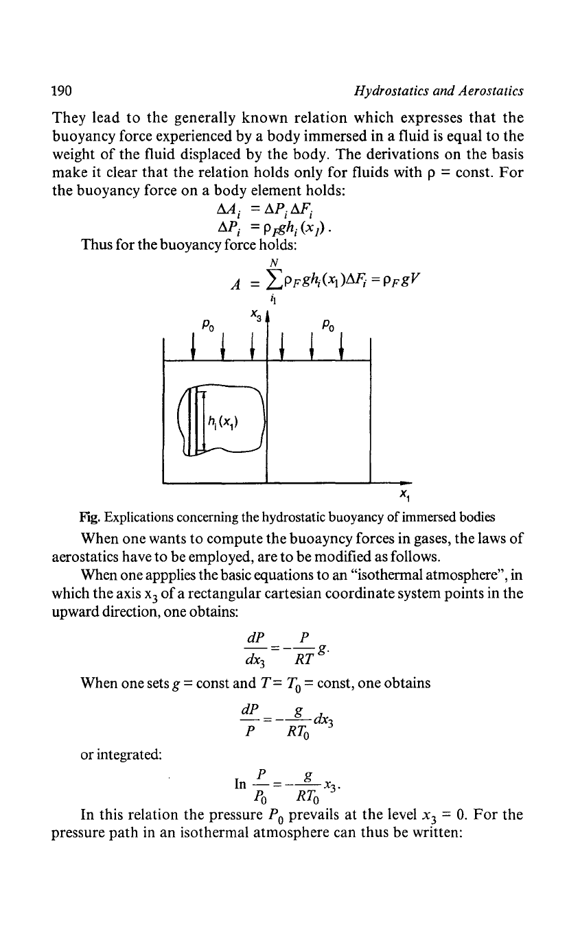
They lead
to
the
generally
known
relation
which expresses
that
the
buoyancy force experienced by a body immersed in a fluid
is
equal
to
the
weight
of
the fluid displaced by the body.
The
derivations
on
the basis
make it clear
that
the relation holds only for fluids with p = const.
For
the buoyancy force
on
a body element holds:
~i
= Il.PillF'i
Il.P
i
= P rfjhi
(x
1)
.
Thus for the buoyancy force holds:
N
A =
LPFgh;(Xl)M;
=PFg
V
X
1
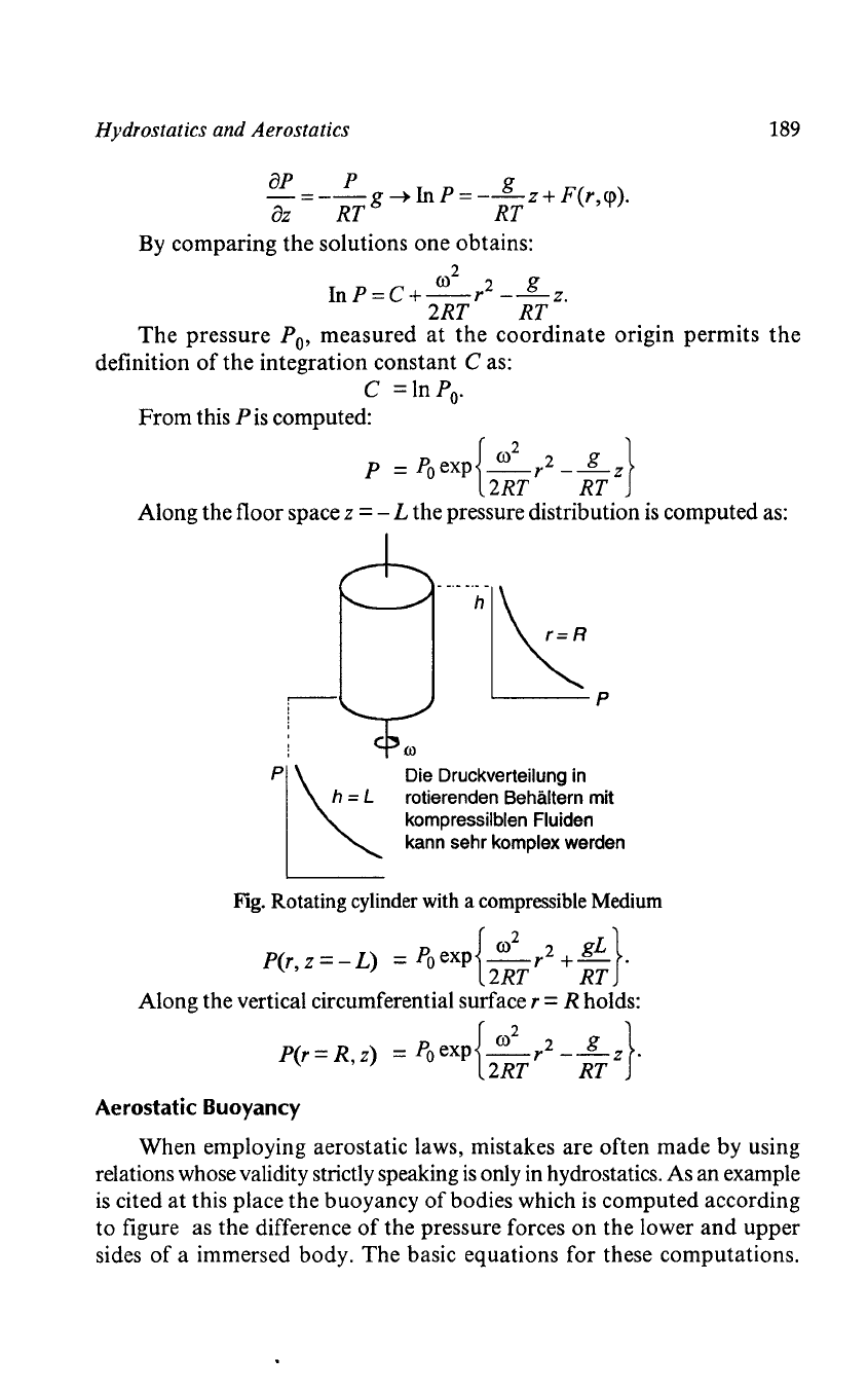
Fig. Explications concerning the hydrostatic buoyancy
of
immersed bodies
When one wants
to
compute the buoayncy forces in gases, the laws
of
aerostatics have to be employed, are to be modified as follows.
When one appplies the basic equations to an
"isothermal atmosphere", in
which the axis
x3
of
a rectangular cartesian coordinate system points in the
upward direction, one obtains:
dP P
-=--g.
dX3
RT
When one sets g = const and
T=
To
= const, one obtains
dP g
-=---
dx3
P
RTo
or integrated:
P g
In
-=---x3'
Po
RTo
In this relation the pressure
Po
prevails at
the
level
x3
=
O.
For
the
pressure
path
in an isothermal atmosphere can thus be written:
Hydrostatics and Aerostatics
P =
poexp{-~X3}
RTo
191
Employing
now
again
the
relation for the buoyancy occurring
on
a
body
element:
M j = !l.P/1F
j
and
writing with employment of(6.116)
M;
=
Po
ex
p
{ -
~;~}
-
Po
ex
p
{-
R~o
(x3i
+ hi)}
i.e.
LV;
~
Po
ex+
~J[
1-
Po
exph~o
iI}]
it becomes quickly evident that for the total buoyancy in the present case,
simple relation stated for p
= const for the total buoyancy force does
not
result.
The
Taylor's series expansion for P
j
can
be
written as:
ap
1 a
2
P 2 1 a
3
P 3
I1P.
=-h
+--h
+--h
+ ...
I a I
28
2
I
683
I
x3
X3
x3
= _
Fog
ex
p
{-
gx3
}h
+
pog2
ex
p
{-
gx3
}h2_
RTo
RTo
I 2R2Tl
RTo
I
[
gh
1
(gh
)2
]
M;~P(x3)gh,
1-
2R~o
+6
R;o
-+
....
Thus
one obtains for the buoyancy force:
A=P(x3)g V - I
1+_
....
[
N
g~2M'.
1
1=1
2RTo
The
first
term
of
this expression (6.123) corresponds
to
the
buoyancy
force
of
hydrostatics.
Conditions for Aerostatics: Stable laminations
A fluid can find itself in mechanical equilibrium (i.e. show no macroscopic
motion) without being in thermal equilibrium. Equation, the condition for the
mechanical equilibrium, can also be given when the temperature in the fluid
is
not
constant. Here the question arises, however, whether such an equilibrium
is
stable.
It
appeared
that
the equilibrium shows the demanded stability only
under
a certain condition.
When
this condition
is
not
met,the static
state
of
the
fluid
is
unstable
and
in the fluid occur flows
of
random
order
which
endeavor to mix the fluid such
that
no constant temperature
is
achieved (in
it). This motion
is
defined as free convection.
The
stability condition for the