Brealey, Myers. Principles of Corporate Finance. 7th edition

Подождите немного. Документ загружается.

Brealey−Meyers:

Principles of Corporate

Finance, Seventh Edition

I. Value 3. How to Calculate

Present Values

Companies, 2003

Calculating PVs and NPVs

You have some bad news about your office building venture (the one described at

the start of Chapter 2). The contractor says that construction will take two years in-

stead of one and requests payment on the following schedule:

1. A $100,000 down payment now. (Note that the land, worth $50,000, must

also be committed now.)

2. A $100,000 progress payment after one year.

3. A final payment of $100,000 when the building is ready for occupancy at

the end of the second year.

Your real estate adviser maintains that despite the delay the building will be worth

$400,000 when completed.

All this yields a new set of cash-flow forecasts:

36 PART I

Value

Period t ⴝ 0 t ⴝ 1 t ⴝ 2

Land ⫺50,000

Construction ⫺100,000 ⫺100,000 ⫺100,000

Payoff ⫹400,000

Total C

⫽⫺150,000 C

⫽⫺100,000 C

⫽⫹300,000

If the interest rate is 7 percent, then NPV is

Table 3.1 calculates NPV step by step. The calculations require just a few key-

strokes on an electronic calculator. Real problems can be much more complicated,

however, so financial managers usually turn to calculators especially programmed

for present value calculations or to spreadsheet programs on personal computers.

In some cases it can be convenient to look up discount factors in present value ta-

bles like Appendix Table 1 at the end of this book.

Fortunately the news about your office venture is not all bad. The contractor is will-

ing to accept a delayed payment; this means that the present value of the contractor’s

fee is less than before. This partly offsets the delay in the payoff. As Table 3.1 shows,

⫽⫺150,000 ⫺

100,000

1.07

⫹

300,000

11.072

NPV ⫽ C

⫹

1 ⫹ r

⫹

11 ⫹ r2

Period Discount Factor Cash Flow Present Value

0 1.0 ⫺150,000 ⫺150,000

1 ⫺100,000 ⫺93,500

2 ⫹300,000 ⫹261,900

Total ⫽ NPV ⫽ $18,400

11.072

⫽ .873

1.07

⫽ .935

TABLE 3.1

Present value worksheet.

Brealey−Meyers:

Principles of Corporate

Finance, Seventh Edition

I. Value 3. How to Calculate

Present Values

Companies, 2003

Sometimes there are shortcuts that make it easy to calculate present values. Let us

look at some examples.

Among the securities that have been issued by the British government are so-

called perpetuities. These are bonds that the government is under no obligation to

repay but that offer a fixed income for each year to perpetuity. The annual rate of

return on a perpetuity is equal to the promised annual payment divided by the

present value:

We can obviously twist this around and find the present value of a perpetuity given

the discount rate r and the cash payment C. For example, suppose that some wor-

thy person wishes to endow a chair in finance at a business school with the initial

payment occurring at the end of the first year. If the rate of interest is 10 percent

and if the aim is to provide $100,000 a year in perpetuity, the amount that must be

set aside today is

How to Value Growing Perpetuities

Suppose now that our benefactor suddenly recollects that no allowance has been

made for growth in salaries, which will probably average about 4 percent a year

starting in year 1. Therefore, instead of providing $100,000 a year in perpetuity, the

benefactor must provide $100,000 in year 1, 1.04 ⫻ $100,000 in year 2, and so on. If

Present value of perpetuity ⫽

⫽

100,000

.10

⫽ $1,000,000

r ⫽

Return ⫽

cash flow

present value

CHAPTER 3 How to Calculate Present Values 37

3.2 LOOKING FOR SHORTCUTS—

PERPETUITIES AND ANNUITIES

We assume the cash flows are safe. If they are risky forecasts, the opportunity cost of capital could be

higher, say 12 percent. NPV at 12 percent is just about zero.

You can check this by writing down the present value formula

···

Now let C/(1 ⫹ r) ⫽ a and 1/(1 ⫹ r) ⫽ x. Then we have (1) PV ⫽ a(1 ⫹ x ⫹ x

⫹ ···).

Multiplying both sides by x, we have (2) PVx ⫽ a(x ⫹ x

⫹ ···).

Subtracting (2) from (1) gives us PV(1 ⫺ x) ⫽ a. Therefore, substituting for a and x,

Multiplying both sides by (1 ⫹ r) and rearranging gives

PV ⫽

PV a1 ⫺

1 ⫹ r

b⫽

1 ⫹ r

PV ⫽

1 ⫹ r

⫹

11 ⫹ r2

⫹

11 ⫹ r2

⫹

the net present value is $18,400—not a substantial decrease from the $23,800 calcu-

lated in Chapter 2. Since the net present value is positive, you should still go ahead.

Brealey−Meyers:

Principles of Corporate

Finance, Seventh Edition

I. Value 3. How to Calculate

Present Values

Companies, 2003

we call the growth rate in salaries g, we can write down the present value of this

stream of cash flows as follows:

Fortunately, there is a simple formula for the sum of this geometric series.

If we

assume that r is greater than g, our clumsy-looking calculation simplifies to

Therefore, if our benefactor wants to provide perpetually an annual sum that keeps

pace with the growth rate in salaries, the amount that must be set aside today is

How to Value Annuities

An annuity is an asset that pays a fixed sum each year for a specified number of

years. The equal-payment house mortgage or installment credit agreement are

common examples of annuities.

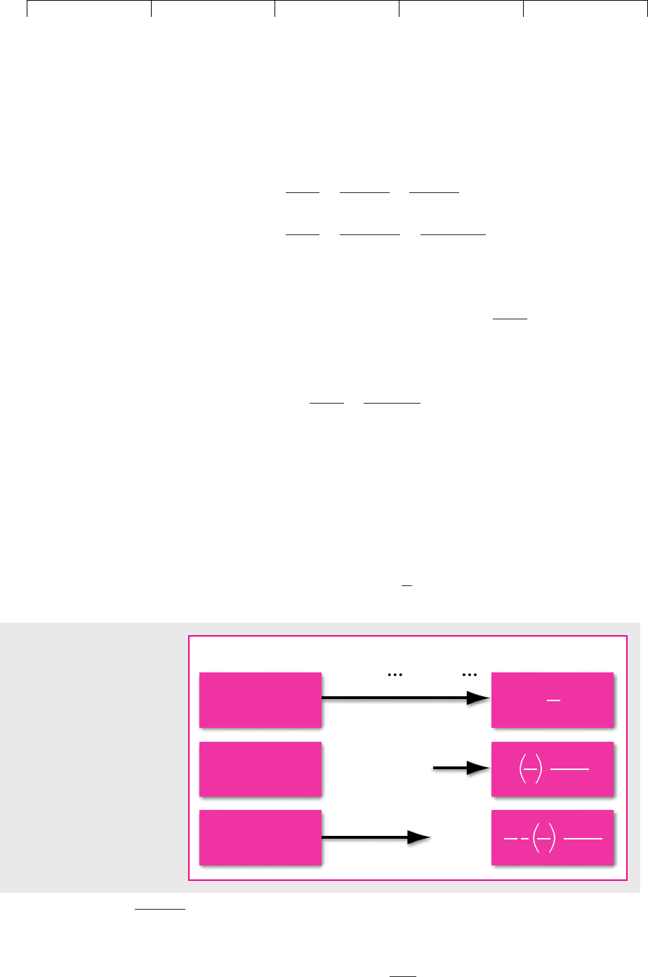
Figure 3.1 illustrates a simple trick for valuing annuities. The first row repre-

sents a perpetuity that produces a cash flow of C in each year beginning in year 1.

It has a present value of

PV ⫽

r ⫺ g

⫽

100,000

.10 ⫺ .04

⫽ $1,666,667

Present value of growing perpetuity ⫽

r ⫺ g

⫽

1 ⫹ r

⫹

11 ⫹ g2

11 ⫹ r2

⫹

11 ⫹ g2

11 ⫹ r2

⫹

…

PV ⫽

1 ⫹ r

⫹

11 ⫹ r2

⫹

11 ⫹ r2

⫹

…

38 PART I Value

We need to calculate the sum of an infinite geometric series PV ⫽ a(1 ⫹ x ⫹ x

⫹ ···) where a ⫽

/(1 ⫹ r) and x ⫽ (1 ⫹ g)/(1 ⫹ r). In footnote 5 we showed that the sum of such a series is a/(1 ⫺ x).

Substituting for a and x in this formula,

PV ⫽

r ⫺ g

Asset Present valueYear of payment

1 2

+ 1

Perpetuity (first

payment year

+1)

(1 +

)

(1 +

)

Annuity from

year 1 to year

Perpetuity (first

payment year 1)

FIGURE 3.1

An annuity that makes

payments in each of years 1 to

t is equal to the difference

between two perpetuities.

Brealey−Meyers:

Principles of Corporate

Finance, Seventh Edition

I. Value 3. How to Calculate

Present Values

Companies, 2003

The second row represents a second perpetuity that produces a cash flow of C in

each year beginning in year t ⫹ 1. It will have a present value of C/r in year t and it

therefore has a present value today of

Both perpetuities provide a cash flow from year t ⫹ 1 onward. The only difference

between the two perpetuities is that the first one also provides a cash flow in each

of the years 1 through t. In other words, the difference between the two perpetu-

ities is an annuity of C for t years. The present value of this annuity is, therefore,

the difference between the values of the two perpetuities:

The expression in brackets is the annuity factor, which is the present value at dis-

count rate r of an annuity of $1 paid at the end of each of t periods.

Suppose, for example, that our benefactor begins to vacillate and wonders what

it would cost to endow a chair providing $100,000 a year for only 20 years. The an-

swer calculated from our formula is

Alternatively, we can simply look up the answer in the annuity table in the Ap-

pendix at the end of the book (Appendix Table 3). This table gives the present value

of a dollar to be received in each of t periods. In our example t ⫽ 20 and the inter-

est rate r ⫽ .10, and therefore we look at the twentieth number from the top in the

10 percent column. It is 8.514. Multiply 8.514 by $100,000, and we have our answer,

$851,400.

Remember that the annuity formula assumes that the first payment occurs

one period hence. If the first cash payment occurs immediately, we would need

to discount each cash flow by one less year. So the present value would be in-

creased by the multiple (1 ⫹ r). For example, if our benefactor were prepared to

make 20 annual payments starting immediately, the value would be $851,400 ⫻

1.10 ⫽ $936,540. An annuity offering an immediate payment is known as an an-

nuity due.

PV ⫽ 100,000 c

.10

⫺

.1011.102

d⫽ 100,000 ⫻ 8.514 ⫽ $851,400

Present value of annuity ⫽ C c

⫺

r11 ⫹ r2

PV ⫽

r11 ⫹ r2

CHAPTER 3 How to Calculate Present Values 39

Again we can work this out from first principles. We need to calculate the sum of the finite geometric

series (1) PV ⫽ a(1 ⫹ x ⫹ x

⫹ ··· ⫹ x

t⫺1

where a ⫽ C/(1 ⫹ r) and x ⫽ 1/(1 ⫹ r).

Multiplying both sides by x, we have (2) PVx ⫽ a(x ⫹ x

⫹ ··· ⫹ x

Subtracting (2) from (1) gives us PV(1 ⫺ x) ⫽ a(1 ⫺ x

Therefore, substituting for a and x,

Multiplying both sides by (1 ⫹ r) and rearranging gives

PV ⫽ C c

⫺

r11 ⫹ r 2

PV a1 ⫺

1 ⫹ r

b⫽ C c

1 ⫹ r

⫺

11 ⫹ r2

t⫹1

Brealey−Meyers:

Principles of Corporate

Finance, Seventh Edition

I. Value 3. How to Calculate

Present Values

Companies, 2003

You should always be on the lookout for ways in which you can use these for-

mulas to make life easier. For example, we sometimes need to calculate how much

a series of annual payments earning a fixed annual interest rate would amass to by

the end of t periods. In this case it is easiest to calculate the present value, and then

multiply it by (1 ⫹ r)

to find the future value.

Thus suppose our benefactor

wished to know how much wealth $100,000 would produce if it were invested each

year instead of being given to those no-good academics. The answer would be

How did we know that 1.10

was 6.727? Easy—we just looked it up in Appendix

Table 2 at the end of the book: “Future Value of $1 at the End of t Periods.”

Future value ⫽ PV ⫻ 1.10

⫽ $851,400 ⫻ 6.727 ⫽ $5.73 million

40 PART I Value

For example, suppose you receive a cash flow of C in year 6. If you invest this cash flow at an interest

rate of r, you will have by year 10 an investment worth C(1 ⫹ r)

. You can get the same answer by cal-

culating the present value of the cash flow PV ⫽ C/(1 ⫹ r)

and then working out how much you would

have by year 10 if you invested this sum today:

Future value ⫽ PV11 ⫹ r 2

⫽

11 ⫹ r2

⫻ 11 ⫹ r2

⫽ C11 ⫹ r 2

3.3 COMPOUND INTEREST AND PRESENT VALUES

There is an important distinction between compound interest and simple interest.

When money is invested at compound interest, each interest payment is reinvested

to earn more interest in subsequent periods. In contrast, the opportunity to earn in-

terest on interest is not provided by an investment that pays only simple interest.

Table 3.2 compares the growth of $100 invested at compound versus simple in-

terest. Notice that in the simple interest case, the interest is paid only on the initial in-

Simple Interest Compound Interest

Starting Ending Starting Ending

Year Balance ⫹ Interest ⫽ Balance Balance ⫹ Interest ⫽ Balance

1 100 ⫹ 10 ⫽ 110 100 ⫹ 10 ⫽ 110

2 110 ⫹ 10 ⫽ 120 110 ⫹ 11 ⫽ 121

3 120 ⫹ 10 ⫽ 130 121 ⫹ 12.1 ⫽ 133.1

4 130 ⫹ 10 ⫽ 140 133.1 ⫹ 13.3 ⫽ 146.4

10 190 ⫹ 10 ⫽ 200 236 ⫹ 24 ⫽ 259

20 290 ⫹ 10 ⫽ 300 612 ⫹ 61 ⫽ 673

50 590 ⫹ 10 ⫽ 600 10,672 ⫹ 1,067 ⫽ 11,739

100 1,090 ⫹ 10 ⫽ 1,100 1,252,783 ⫹ 125,278 ⫽ 1,378,061

200 2,090 ⫹ 10 ⫽ 2,100 17,264,116,042 ⫹ 1,726,411,604 ⫽ 18,990,527,646

226 2,350 ⫹ 10 ⫽ 2,360 205,756,782,755 ⫹ 20,575,678,275 ⫽ 226,332,461,030

TABLE 3.2

Value of $100 invested at 10 percent simple and compound interest.

Brealey−Meyers:

Principles of Corporate

Finance, Seventh Edition

I. Value 3. How to Calculate

Present Values

Companies, 2003

vestment of $100. Your wealth therefore increases by just $10 a year. In the com-

pound interest case, you earn 10 percent on your initial investment in the first year,

which gives you a balance at the end of the year of 100 ⫻ 1.10 ⫽ $110. Then in the

second year you earn 10 percent on this $110, which gives you a balance at the end

of the second year of 100 ⫻ 1.10

⫽ $121.

Table 3.2 shows that the difference between simple and compound interest is

nil for a one-period investment, trivial for a two-period investment, but over-

whelming for an investment of 20 years or more. A sum of $100 invested during

the American Revolution and earning compound interest of 10 percent a year

would now be worth over $226 billion. If only your ancestors could have put

away a few cents.

The two top lines in Figure 3.2 compare the results of investing $100 at 10 per-

cent simple interest and at 10 percent compound interest. It looks as if the rate of

growth is constant under simple interest and accelerates under compound interest.

However, this is an optical illusion. We know that under compound interest our

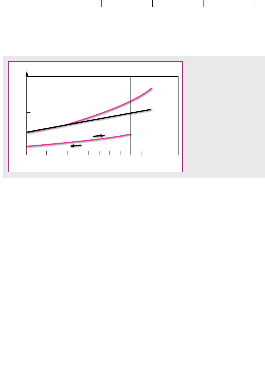
wealth grows at a constant rate of 10 percent. Figure 3.3 is in fact a more useful pre-

sentation. Here the numbers are plotted on a semilogarithmic scale and the con-

stant compound growth rates show up as straight lines.

Problems in finance almost always involve compound interest rather than sim-

ple interest, and therefore financial people always assume that you are talking

about compound interest unless you specify otherwise. Discounting is a process of

compound interest. Some people find it intuitively helpful to replace the question,

What is the present value of $100 to be received 10 years from now, if the opportu-

nity cost of capital is 10 percent? with the question, How much would I have to in-

vest now in order to receive $100 after 10 years, given an interest rate of 10 percent?

The answer to the first question is

PV ⫽

100

11.102

⫽ $38.55

CHAPTER 3 How to Calculate Present Values 41

Dollars

300

200

100

38.55

2 3 4 5 6 7 8 9 10 11 Future time,

years

Growth at

compound

interest

(10%)

Growth at

simple

interest

(10%)

Growth at compound interest

Discounting at 10%

100

200

259

FIGURE 3.2

Compound interest versus simple

interest. The top two ascending

lines show the growth of $100

invested at simple and compound

interest. The longer the funds

are invested, the greater the

advantage with compound

interest. The bottom line shows

that $38.55 must be invested now

to obtain $100 after 10 periods.

Conversely, the present value of

$100 to be received after 10 years

is $38.55.

Brealey−Meyers:

Principles of Corporate

Finance, Seventh Edition

I. Value 3. How to Calculate

Present Values

Companies, 2003

And the answer to the second question is

The bottom lines in Figures 3.2 and 3.3 show the growth path of an initial invest-

ment of $38.55 to its terminal value of $100. One can think of discounting as trav-

eling back along the bottom line, from future value to present value.

A Note on Compounding Intervals

So far we have implicitly assumed that each cash flow occurs at the end of the year.

This is sometimes the case. For example, in France and Germany most corporations

pay interest on their bonds annually. However, in the United States and Britain

most pay interest semiannually. In these countries, the investor can earn an addi-

tional six months’ interest on the first payment, so that an investment of $100 in a

bond that paid interest of 10 percent per annum compounded semiannually would

amount to $105 after the first six months, and by the end of the year it would

amount to 1.05

⫻ 100 ⫽ $110.25. In other words, 10 percent compounded semian-

nually is equivalent to 10.25 percent compounded annually.

Let’s take another example. Suppose a bank makes automobile loans requiring

monthly payments at an annual percentage rate (APR) of 6 percent per year. What

does that mean, and what is the true rate of interest on the loans?

With monthly payments, the bank charges one-twelfth of the APR in each

month, that is, 6/12 ⫽ .5 percent. Because the monthly return is compounded, the

Investment ⫽

100

11.102

⫽ $38.55

Investment ⫻ 11.102

⫽ $100

42 PART I

Value

Dollars, log scale

200

100

38.55

234567891011

Future time,

years

Growth at

compound

interest

(10%)

Growth at

simple

interest

(10%)

Growth at compound interest

Discounting at 10%

100

400

FIGURE 3.3

The same story as Figure 3.2,

except that the vertical scale is

logarithmic. A constant

compound rate of growth

means a straight ascending

line. This graph makes clear

that the growth rate of funds

invested at simple interest

actually declines as time

passes.

Brealey−Meyers:

Principles of Corporate

Finance, Seventh Edition

I. Value 3. How to Calculate

Present Values

Companies, 2003

bank actually earns more than 6 percent per year. Suppose that the bank starts

with $10 million of automobile loans outstanding. This investment grows to

$10 ⫻ 1.005 ⫽ $10.05 million after month 1, to $10 ⫻ 1.005

⫽ $10.10025 million

after month 2, and to $10 ⫻ 1.005

⫽ $10.61678 million after 12 months.

Thus the

bank is quoting a 6 percent APR but actually earns 6.1678 percent if interest pay-

ments are made monthly.

In general, an investment of $1 at a rate of r per annum compounded m times a

year amounts by the end of the year to [1 ⫹ (r/m)]

, and the equivalent annually

compounded rate of interest is [1 ⫹ (r/m)]

⫺ 1.

Continuous Compounding The attractions to the investor of more frequent pay-

ments did not escape the attention of the savings and loan companies in the 1960s

and 1970s. Their rate of interest on deposits was traditionally stated as an annually

compounded rate. The government used to stipulate a maximum annual rate of in-

terest that could be paid but made no mention of the compounding interval. When

interest ceilings began to pinch, savings and loan companies changed progres-

sively to semiannual and then to monthly compounding. Therefore the equivalent

annually compounded rate of interest increased first to [1 ⫹ (r/2)]

⫺ 1 and then

to [1 ⫹ (r/12)]

⫺ 1.

Eventually one company quoted a continuously compounded rate, so that pay-

ments were assumed to be spread evenly and continuously throughout the year. In

terms of our formula, this is equivalent to letting m approach infinity.

This might

seem like a lot of calculations for the savings and loan companies. Fortunately,

however, someone remembered high school algebra and pointed out that as m ap-

proaches infinity [1 ⫹ (r/m)]

approaches (2.718)

. The figure 2.718—or e, as it is

called—is simply the base for natural logarithms.

One dollar invested at a continuously compounded rate of r will, therefore,

grow to e

⫽ (2.718)

by the end of the first year. By the end of t years it will grow

to e

⫽ (2.718)

. Appendix Table 4 at the end of the book is a table of values of e

Let us practice using it.

Example 1 Suppose you invest $1 at a continuously compounded rate of 11 per-

cent (r ⫽ .11) for one year (t ⫽ 1). The end-year value is e

.11

, which you can see from

the second row of Appendix Table 4 is $1.116. In other words, investing at 11 per-

cent a year continuously compounded is exactly the same as investing at 11.6 per-

cent a year annually compounded.

Example 2 Suppose you invest $1 at a continuously compounded rate of 11 per-

cent (r ⫽ .11) for two years (t ⫽ 2). The final value of the investment is e

⫽ e

.22

. You

can see from the third row of Appendix Table 4 that e

.22

is $1.246.

CHAPTER 3

How to Calculate Present Values 43

Individual borrowers gradually pay off their loans. We are assuming that the aggregate amount loaned

by the bank to all its customers stays constant at $10 million.

Unfortunately, U.S. truth-in-lending laws require lenders to quote interest rates for most types of con-

sumer loans as APRs rather than true annual rates.

When we talk about continuous payments, we are pretending that money can be dispensed in a con-

tinuous stream like water out of a faucet. One can never quite do this. For example, instead of paying

out $100,000 every year, our benefactor could pay out $100 every 8

⁄4 hours or $1 every 5

⁄4 minutes or

1 cent every 3

⁄6 seconds but could not pay it out continuously. Financial managers pretend that payments

are continuous rather than hourly, daily, or weekly because (1) it simplifies the calculations, and (2) it

gives a very close approximation to the NPV of frequent payments.

Brealey−Meyers:

Principles of Corporate

Finance, Seventh Edition

I. Value 3. How to Calculate

Present Values

Companies, 2003

There is a particular value to continuous compounding in capital budgeting,

where it may often be more reasonable to assume that a cash flow is spread evenly

over the year than that it occurs at the year’s end. It is easy to adapt our previous

formulas to handle this. For example, suppose that we wish to compute the pres-

ent value of a perpetuity of C dollars a year. We already know that if the payment

is made at the end of the year, we divide the payment by the annually compounded

rate of r:

If the same total payment is made in an even stream throughout the year, we use

the same formula but substitute the continuously compounded rate.

Example 3 Suppose the annually compounded rate is 18.5 percent. The present

value of a $100 perpetuity, with each cash flow received at the end of the year, is

100/.185 ⫽ $540.54. If the cash flow is received continuously, we must divide $100

by 17 percent, because 17 percent continuously compounded is equivalent to

18.5 percent annually compounded (e

.17

⫽ 1.185). The present value of the contin-

uous cash flow stream is 100/.17 ⫽ $588.24.

For any other continuous payments, we can always use our formula for valuing

annuities. For instance, suppose that our philanthropist has thought more seri-

ously and decided to found a home for elderly donkeys, which will cost $100,000

a year, starting immediately, and spread evenly over 20 years. Previously, we used

the annually compounded rate of 10 percent; now we must use the continuously

compounded rate of r ⫽ 9.53 percent (e

.0953

⫽ 1.10). To cover such an expenditure,

then, our philanthropist needs to set aside the following sum:

Alternatively, we could have cut these calculations short by using Appendix Table 5.

This shows that, if the annually compounded return is 10 percent, then $1 a year

spread over 20 years is worth $8.932.

If you look back at our earlier discussion of annuities, you will notice that the

present value of $100,000 paid at the end of each of the 20 years was $851,400.

⫽ 100,000 a

.0953

⫺

.0953

⫻

6.727

b⫽ 100,000 ⫻ 8.932 ⫽ $893,200

PV ⫽ C a

⫺

⫻

PV ⫽

44 PART I Value

Remember that an annuity is simply the difference between a perpetuity received today and a per-

petuity received in year t. A continuous stream of C dollars a year in perpetuity is worth C/r, where r

is the continuously compounded rate. Our annuity, then, is worth

Since r is the continuously compounded rate, C/r received in year t is worth (C/r) ⫻ (1/e

) today. Our

annuity formula is therefore

sometimes written as

11 ⫺ e

⫺rt

PV ⫽

⫺

⫻

PV ⫽

⫺ present value of

received in year t

Brealey−Meyers:

Principles of Corporate

Finance, Seventh Edition

I. Value 3. How to Calculate

Present Values

Companies, 2003

Therefore, it costs the philanthropist $41,800—or 5 percent—more to provide a

continuous payment stream.

Often in finance we need only a ballpark estimate of present value. An error of

5 percent in a present value calculation may be perfectly acceptable. In such cases

it doesn’t usually matter whether we assume that cash flows occur at the end of the

year or in a continuous stream. At other times precision matters, and we do need

to worry about the exact frequency of the cash flows.

CHAPTER 3

How to Calculate Present Values 45

3.4 NOMINAL AND REAL RATES OF INTEREST

If you invest $1,000 in a bank deposit offering an interest rate of 10 percent, the

bank promises to pay you $1,100 at the end of the year. But it makes no promises

about what the $1,100 will buy. That will depend on the rate of inflation over the

year. If the prices of goods and services increase by more than 10 percent, you have

lost ground in terms of the goods that you can buy.

Several indexes are used to track the general level of prices. The best known is the

Consumer Price Index, or CPI, which measures the number of dollars that it takes to

pay for a typical family’s purchases. The change in the CPI from one year to the next

measures the rate of inflation. Figure 3.4 shows the rate of inflation in the United

1930

–15

–5

–10

1940 1950 1960 1970 1980 1990 2000

Annual inflation, percent

FIGURE 3.4

Annual rates of inflation in the United States from 1926 to 2000.

Source: Ibbotson Associates, Inc., Stocks, Bonds, Bills, and Inflation, 2001 Yearbook, Chicago, 2001.