Blank B.E., Krantz S.G. Calculus: Single Variable

Подождите немного. Документ загружается.

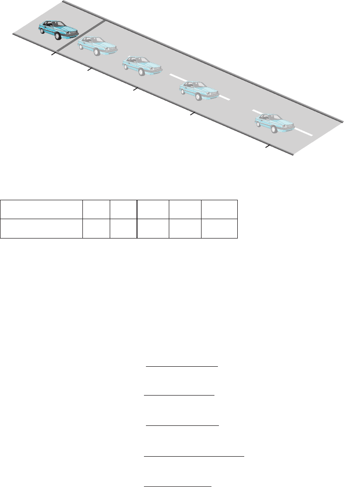
Time (seconds) 01 2 3 4

Distance (feet) 083272128

Table 3.2

This

calculation gives a rough approximation to the velocity at time t 5 1 but does

not tell us the exact velocity at the instant t 5 1. However, it suggests an

idea: instead of calculating average velocity over a long time interval (of length

one second), let us calculate average velocity over a short time interval. This

should give a better approximation to the velocity at the instant t 5 1. We will use

the symbol Δt to denote the elapsed time. Over the time interval from t 5 1to

t 5 1 1 Δt, car B travels from p(1) to p(1 1 Δt). The average velocity in ft/s is then

rate 5

distance traveled

elapsed time

pð1 1 ΔtÞ2 pð1Þ

Δt

8ð11ΔtÞ

2 8  1

Δt

8 1 16  Δt 1 8ðΔtÞ

2 8

Δt

16  Δt 1 8ðΔtÞ

Δt

5 16 1 8ðΔtÞ:

We have found that the average velocity over the time interval from t 5 1to

t 5 11Δt is equal to 16 1 8(Δt) feet per second. Notice that if we let Δt tend to 0,

then the average velocity, 16 1 8(Δt) ft/s, has a limit: 16 ft/s. It is therefore reasonable

to say that the velocity of car B at the instant t 5 1 is the limit of the average velocity

over the time interval from t 5 1tot 5 1 1 Δt as Δt - 0. With this deﬁnition, the

velocity of car B at t 5 1 is lim

Δt-0

(16 1 8(Δt)) ft/s, or 16 ft/s.

128

t  0

t  1

t  2

t  3

t  4

m Figure 2

3.1 Rates of Change and Tangent Lines 165

The Deﬁnition of

Instantaneous Velocity

We now summarize our investigation of instantaneous velocity with a deﬁnition.

DEFINITION

Suppose that the position of a body moving along an axis is

described by a function p of time t.Theinstantaneous velocity of the body at

time c is

lim

Δt-0

pðc 1 ΔtÞ2 pðcÞ

Δt

;

provided that this limit exists and is ﬁnite.

For ease of reference, we denote the instantaneous velocity at time c by

ðcÞ. Thus

ðcÞ5 lim

Δt-0

pðc 1 ΔtÞ2 pðcÞ

Δt

: ð3:1:1Þ

Our ﬁrst two examples show that limit formula (3.1.1) agrees with our intuitive

understanding of veloc ity in some simple situations.

⁄ EX

AMPLE 1 Let α be a constant. Suppose that the position of car C is

given by p(t) 5 α ft for all values of t. Because p(t) is constant, car C is not moving.

Common sense tells us that its velocity is 0 at every instant c. Verify that formula

(3.1.1) leads to the same conclusion.

Solution Let c denote

any instant of time. We calculate:

ðcÞ5 lim

Δt-0

pðc 1 ΔtÞ2 pðtÞ

Δt

5 lim

Δt-0

α 2 α

Δt

5 lim

Δt-0

Δt

5 lim

Δt-0

0 5 0 ¥

⁄ EXAMPLE 2 Suppose that the position of car A is

given in feet by 50t when

t is measured in seconds (as in Table 1). Verify that the instantaneous velocity of

car A is 50 feet per second for every value of t.

Solution Because p(t) 5 50t feet,

the instantaneous velocity in feet per second at

time t 5 c is

ðcÞ 5 lim

Δt-0

pðc 1 ΔtÞ2 pðcÞ

Δt

5 lim

Δt-0

50ðc 1 ΔtÞ2 50c

Δt

5 lim

Δt-0

50Δt

Δt

5 lim

Δt-0

5 50: ¥

INSIGHT

In Example 2 it is useful to notice that we can replace p(t) 5 50t with

p(t) 5 αt where α is an arbitrary constant. By doing so we see that

If pðtÞ5 αt ; with α constant; then p

ðcÞ5 α: ð3:1:2Þ

Our next two examples call for velocity calculations that require the precise

deﬁnition of instantaneous velocity, as given by formula (3.1.1).

166 Chapter 3 The Derivative

⁄ EXAMPLE 3 As in the discussion at the beginning of this section, the

position of car B is given by p(t) 5 8t

. What is its velocity when t 5 1? When t 5 2?

Solution By

formula (3.1.1), the instantaneous velocity of car B at time t 5 c is

ðcÞ 5 lim

Δt-0

pðc 1 ΔtÞ2 pðcÞ

Δt

5 lim

Δt-0

8ðc 1 ΔtÞ

2 8c

Δt

5 8  lim

Δt-0



1 2cΔt 1 ðΔtÞ



2 c

Δt

5 8  lim

Δt-0

ð2c 1 ΔtÞ

5 8  2c:

If we set c 5 1 in this formula for p

ðcÞ, then we arrive at p

ð1Þ5 16, which agrees

with the value we obtained in the discussion at the beginning of this section. In this

example, however, we have done much more. By calculating p

ðcÞ for a general

value c, we can state the velocity of car B at any other time with no extra work.

Thus to calculate the velocity of car B when t 5 2, we set c 5 2 in our formula for

ðcÞ and obtain 8 2 2, or 32. ¥

INSIGHT

In Example 3, it is useful to notice that we can replace p(t) 5 8t

with

p(t) 5 αt

where α is an arbitrary constant. By repeating the calculation with the arbitrary

constant α instead of the speciﬁc constant 8, we see that

If pðtÞ5 αt

; with α constant; then p

ðcÞ5 α  2c: ð3:1:3Þ

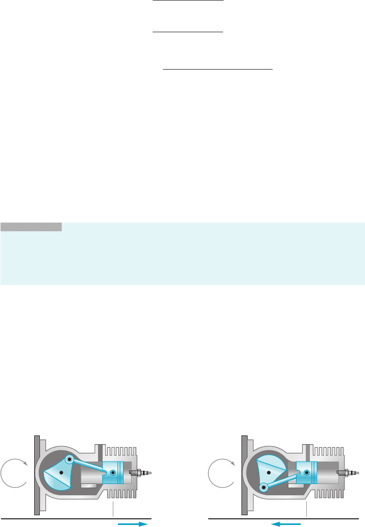
⁄ EXAMPLE 4 Relative to a speciﬁed horizontal coordinate system, the

position of a point Q on a piston is given by

pðtÞ5 18 1 4t 2 2t

;

in inches, for 0 # t # 4 seconds. See Figure 3. What is the instantaneous velocity

of the piston at time t 5 3?

t  3

m Figure 3b Negative velocity

m Figure 3a Positive velocity

3.1 Rates of Change and Tangent Lines 167

Solution Because p(t) is measured in inches and t in seconds, we see from formula

(3.1.1) that the units of p

ð3Þ will be inches per second. We calculate p(3) 5 18 1

4 3 2 2 3

5 12 and

pð3 1 ΔtÞ 5 18 1 4ð3 1 ΔtÞ2 2ð31ΔtÞ

5 18 1 12 1 4Δt 2 2



9 1 6Δt 1 ðΔtÞ



5 12 2 8Δt 2 2ðΔtÞ

Therefore

ð3Þ 5 lim

Δt-0

pð3 1 ΔtÞ2 pð3Þ

Δt

5 lim

Δt-0



12 2 8Δ t 2 2ðΔtÞ



2 12

Δt

5 lim

Δt-0

2 8Δt 2 2ðΔtÞ

Δt

5 lim

Δt-0

ð2 8 2 2ΔtÞ

528:

Thus p

ð3Þ528 in/s.

INSIGHT

The meaning of negative velocity of an object can be understood by

looking at the deﬁnition of velocity. If Δt . 0, then the average velocity

pðc 1 ΔtÞ2 pðcÞ

Δt

at time t 5 c will be positive if



pðc 1 ΔtÞ2 pðcÞ



. 0 (the object is moving forward)

and negative if



pðc 1 ΔtÞ2 pðcÞ



, 0 (the object is moving backward). Passing to the

limit, we see that positive instantaneous velocity corresponds to forward motion whereas

negative instantaneous velocity corresponds to backward motion. In Example 4, the

piston is moving to the left (in the negative direction in the coordinate system) at the

instant t 5 3 (see Figure 3b). In everyday speech, we do not distinguish between speed

and velocity. In mathematics and physics, however, speed refers to the absolute value of

velocity. Thus speed is always nonnegative.

Instantaneous Rate of

Change

We have just deﬁned instantaneous velocity as a limit of average velocities. It is

useful to extend this construction to other functions f. In the present discussion, we

do not assume that the variable x represents time. Additionally, the expression f (x)

is not assumed to be a distance. Whatever quantities x and f (x) do measure, it is

still true that the quotient

f ðc 1 Δ x Þ2 f ðcÞ

Δx

is the average rate of change of f (x)asx changes from c to c1 Δ x. By letting

Δx - 0, we obtain the instantaneous rate of change f

ðcÞ of f (x)atx 5 c:

ðcÞ5 lim

Δx-0

f ðc 1 Δ x Þ2 f ðcÞ

Δx

; ð3:1:4Þ

provided this limit exists and is ﬁnite.

168 Chapter 3 The Derivative

Notice that the limits in formulas (3.1.1) and (3.1.4) are mathematically the

same. That is because instantaneous velocity is a particular example of the

instantaneous rate of change of a function. Other instantaneous rates of change

often are of interest. In economics, the function f (x) of formula (3.1.4) might be the

cost of producing x units of a commodity. In that case, the instantaneous rate of

change f

ðcÞ is called the marginal cost of producing the c

unit. In pharmacology,

f (x) might be the measurable effect of a drug on a patient at time x. The instan-

taneous rate of change f

ðcÞ would then be called the sensitivity of the patient to the

drug at time c.

⁄ EX

AMPLE 5 The volume of a sphere of radius r is 4πr

=3. What is the

instantaneous rate of change of the volume with respect to r when r 5 3?

Solution The

volume f (r) of a sphere of radius r is given by f ðrÞ5 4πr

=3. Let us

denote the constant 4π/3 by α for short, so that f ðrÞ5 αr

. We are required to

calculate f

ð3Þ. We will carry out the calculation for a general value c of r and

answer the question by substituting c 5 3. To do so, we refer to formula (3.1.4). It is

more natural to continue using the variable r for the radius rather than switching

to x. Letting Δr denote the increment in the radius, we have

ðcÞ5 lim

Δr-0

f ðc 1 Δ rÞ2 f ðcÞ

Δr

5 lim

Δr-0

αðc1ΔrÞ

2 αc

Δr

5 α lim

Δr-0



1 3c

 Δr 1 3cðΔrÞ

1 ðΔrÞ



2 c

Δr

Because the numerator simpliﬁes to 3c

 Δr 1 3cðΔrÞ

1 ðΔrÞ

,or

ðΔrÞ



1 3cðΔrÞ1 ðΔrÞ



, it follows that

ðcÞ5 α lim

Δr-0

ðΔrÞ



1 3cðΔrÞ1 ðΔrÞ



Δr

5 α lim

Δr-0



1 3cðΔrÞ1 ðΔrÞ



5 α  3c

In summary:

If f ðxÞ5 αx

with α constant; then f

ðcÞ5 α  3 c

: ð3:1:5Þ

Because α 5 4 π=3; we see that

ðcÞ5

4π

 3c

5 4πc

Thus f

ð3Þ5 4π  3

5 36π is the instantaneous rate of change of volume with

respect to r when r 5 3.

b A LOOK BACK Examples 1, 2, 3, and 5 are concerned with the instantaneous rates

of change of functions of the form f (x) 5 αx

for n 5 0, 1, 2, and 3. A careful

examination reveals that there is a pattern to the formulas for f

ðcÞ. The key is

to restate line (3.1.5) as follows: If α is a constant, if n 5 3, and if f ðxÞ5 αx

3.1 Rates of Change and Tangent Lines 169

then f

ðcÞ5 α  nc

n21

: Lines (3.1.3) and (3.1.2) show that this relationship between

f and f

also holds for n 5 2 and n 5 1, respectively. Furthermore, if we set n 5 0,

then f ðxÞ5 αx

5 αx

5 α is the constant function α,andf

ðcÞ5 α  nc

n21

α  0  c

n21

5 0 is the function that is identically 0. In Example 1, we veriﬁed that the

instantaneous rate of change of a constant function is 0. Thus the rule we

have found for f

holds when n 5 0. In summary:

If f ðxÞ5 α  x

for n 5 0; 1; 2; or 3; then f

ðcÞ5 α  nc

n1

ð3:1:6Þ

Sums of Functions Our next theorem tells us that, if α is a constant, then the instantaneous rate of

change of (αf )(x)isα times the instantaneous rate of change of f (x). It also tells us

that we can calculate the instantaneous rate of change of a sum by adding the

instantaneous rates of change of its summands.

THEOREM 1

Suppose that f

ðcÞand g

ðcÞexist, and that α and β are constants. Then

ðαf Þ

ðcÞ5 α  f

ðcÞ; ð3:1:7Þ

ðf 1 gÞ

ðcÞ5 f

ðcÞ1 g

ðcÞ; ð3:1:8Þ

and, more generally,

ðα  f 1 β  gÞ

ðcÞ5 α  f

ðcÞ1 β  g

ðcÞ: ð3:1:9Þ

Proof. Wh

en we calculate an instantaneous rate of change using deﬁnition (3.1.4),

we are evaluating a limit. We therefore make use of appropriate limit laws. Thus to

calculate

ðα  f 1 β  gÞ

ðcÞ

we use parts (a) and (d) of Theorem 2, Section 2.2:

ðα  f 1 β  gÞ

ðcÞ5 lim

Δx-0

ðα  f 1 β  gÞðc 1 ΔxÞðα  f 1 β  gÞðcÞ

Δx

5 lim

Δx-0



f ðc 1 Δ x Þf ðcÞ



1 β



gðc 1 ΔxÞgðcÞ



Δx

rearranging terms

5 lim

Δx-0



f ðc 1 Δ x Þf ðcÞ



Δx

1 lim

Δx-0



gðc 1 ΔxÞgðcÞ



Δx

using Theorem 2a; Section 2:2

5 α  lim

Δx-0

f ðc 1 Δ x Þf ðcÞ

Δx

1 β  lim

Δx-0

gðc 1 ΔxÞgðcÞ

Δx

using Theorem 2d; Section 2:2

5 α  f

ðcÞ1 β  g

ðcÞ by definition ð3:1:4Þ;

which proves (3.1.9). Equation (3.1.8) is the special case of (3.1.9) that results

from setting α 5 β 5 1. Equation (3.1.7) is the special case of (3.1.9) that results from

setting β 5 0. ’

170 Chapter 3 The Derivative

⁄ EXAMPLE 6 What is the instantaneous rate of change of FðxÞ5 7x

2 5x

at x 521?

Solution We

are asked for F

(21). Equation (3.1.4) deﬁnes this quantity as a limit,

but we now have several rules that allow us to calculate instantaneous rate of

change witho ut referring to the limit process. Let f ðxÞ5 7x

and gðxÞ525x

. Then

F(x) 5 f (x) 1 g(x). By equation (3.1.6) with α 5 7 and n 5 3, we have f

ð2 1Þ5

7  3ð21Þ

321

5 21: By equation (3.1.6) with α 525 and n 5 2, we have

ð2 1Þ5 ð2 5Þ2ð21Þ

221

5 10: Thus by applying equation (3.1.8), we obtain

ð2 1Þ5 21 1 10 5 31: ¥

We can easily extend formulas (3.1.8) and (3.1.9) to three or more summands. For

example, by applying (3.1.8) twice, we can handle the sum of three terms as follows:

ðf 1 g 1 hÞ

ðcÞ5



ðf 1 gÞ1 h



ðcÞ5 ðf 1 gÞ

ðcÞ1 h

ðcÞ5 f

ðcÞ1 g

ðcÞ1 h

ðcÞ:

ð3:1:10Þ

⁄ EX

AMPLE 7 Let p(t) 5 18 1 4t 2 2 t

. In Example 4, we obtained p

ð3Þ528

by evaluating a limit. Derive this result by using equations (3.1.6) and (3.1.10)

instead.

Solution Let f ðtÞ5 18 5 18t

, gðt Þ5 4t 5 4 t

, and hðtÞ522t

. According to

equation (3.1.6), we have f

ð3Þ5 18  0 ð3Þ

021

5 0, g

ð3Þ5 4  1 ð3Þ

121

5 4, and

ð3Þ5 ð22Þ2 ð3Þ

221

5212. Therefore by equation (3.1.10), we have

ð3Þ5 0 1 4 1 ð212Þ528. ¥

The Concept of

Tangent Line

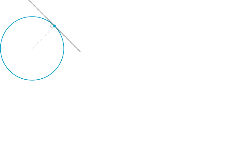
It is easy to understand the idea of the tangent line to a circle. Here are three good

ways to think about the tangent line to the circle C at the point P (illustrated in

Figure 4).

1. The tangent line is perpendicular to the radius at P and passes through P.

2. The tangent line passes through P and intersects C at just that one point.

3. The tangent line passes through P, and the circle lies on one side of the tangent

line.

All of these descriptions are correct, and all of them uniquely determine the

tangent line to the circle C at the point P. But each of them is useless in deter-

mining the tangent line to the curve in Figure 5 at the point P. Intuition tells us that

the dotted line in the ﬁgure is the tangent line. But this line in no sense satisﬁes

statements 1, 2, or 3; we need a new mathematical description of tangent line.

We use a limiting process to determine the tangent line to the graph of y 5 f (x)

at a point P 5



c; f ðcÞ



. Consider the graph in Figure 5. The dotted line indicates

what our intuition tells us that the tangent line is—the dotted line through P that

“most nearly approximates” the curve. The trouble is that it takes two pieces of

information to determine a line. We only know one: the point P through which the

line passes. We get a second piece of information, namely the slope m, by considering

nearby secant lines, such as the line passing through points P and P

in Figure 6.

A secant line is a line passing through two points of the curve—in this case P 5



c; f ðcÞ



and P



c 1 Δx; f



c 1 ΔxÞ



. The slope of this secant line is

f ðc 1 Δ x Þ2 f ðcÞ

ðc 1 ΔxÞ2 c

; or

f ðc 1 ΔxÞ2 f ðcÞ

Δx

Tangent line

m Figure 4

3.1 Rates of Change and Tangent Lines 171

What we see geometrically is that, as Δx - 0 (that is, as P

-P), the slope of the

secant line tends to the slope of the tangent line at P. In other words, we are saying

that the slope m of the tangen t line to y 5 f (x)atP 5



c; f ðcÞ



is given by

m 5 lim

Δx-0

f ðc 1 ΔxÞ2 f ðcÞ

Δx

: ð3:1:11Þ

Refer to Figure 7.

INSIGHT

Observe that the right side of equation (3.1.11) is identical to the right side

of equation (3.1.4). That is, the slope of the tangent line to the graph of f at



c; f ðcÞ



the same as the instantaneous rate of change of f (x) with respect to x at x 5 c. This

may seem surprising at ﬁrst—especially when f (x) has some other physical meaning

(such as volume, as in Example 5). But when we graph the equation y 5 f (x), the value

f (x), in addition to any other meaning it may have, represents the distance of the point



x; f ðxÞ



from the x-axis. The increment f ðc 1 ΔxÞ2 f ðcÞ is therefore a vertical increment

Δy, and the quotient

f ðc 1 ΔxÞ2 f ðcÞ

Δx

is a slope

Δy

Δx

. Thus f

ðcÞ is both an instantaneous

rate of change of f and a slope.

Using the point-slope equation of a lin e (Section 1.3) and formula (3.1.11), we

may now deﬁne the tangent line to the graph of a function at a point.

DEFINITION

Let f be deﬁned on an open interval containing the point c.

Suppose that the limit

ðcÞ5 lim

Δx-0

f ðc 1 ΔxÞ2 f ð cÞ

Δx

exists and is ﬁnite. Then the tangent line to the graph of f at the point (c, f (c))

is the line with Cartesian equation

y 5 f

ðcÞðx 2 cÞ1 f ðcÞ: ð3:1:12Þ

In particular,

ðcÞ5 the slope of the tangent line to the graph of f at the point



c; f ðcÞ



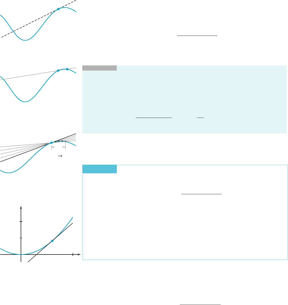
⁄ EX

AMPLE 8 Find the equation of the tangent line to the graph of y 5 x

the point P 5 (3, 9).

Solution Let f (x) 5 x

. The slope of the tangent line at P 5 (3, 9) is

ð3Þ5 lim

Δx-0

f ð3 1 ΔxÞ2 f ð3Þ

Δx

To evaluate this limit, we can use line (3.1.6) with α 5 1, n 5 2, and c 5 3. We

obtain f

ð3Þ5 1 2 (3

) 5 6. According to formu la (3.1.12), the equation of the

tangent line is y 5 6(x 2 3) 1 9. The graph of f and its tangent line are shown in

Figure 8.

y  6

(

x  3

)

 9

y  x

P  (3, 9)

m Figure 8 From the tickmarks,

notice that the axes have different

scales. That is why the slope of

the tangent line, which is actually

6, appears to be close to 1.

x

x 0

y  f

(

)

Tangent line

Secant lines

m Figure 7

y  f(x)

Secant line

m Figure 6

y  f(x)

m Figure 5

172 Chapter

3 The Derivative

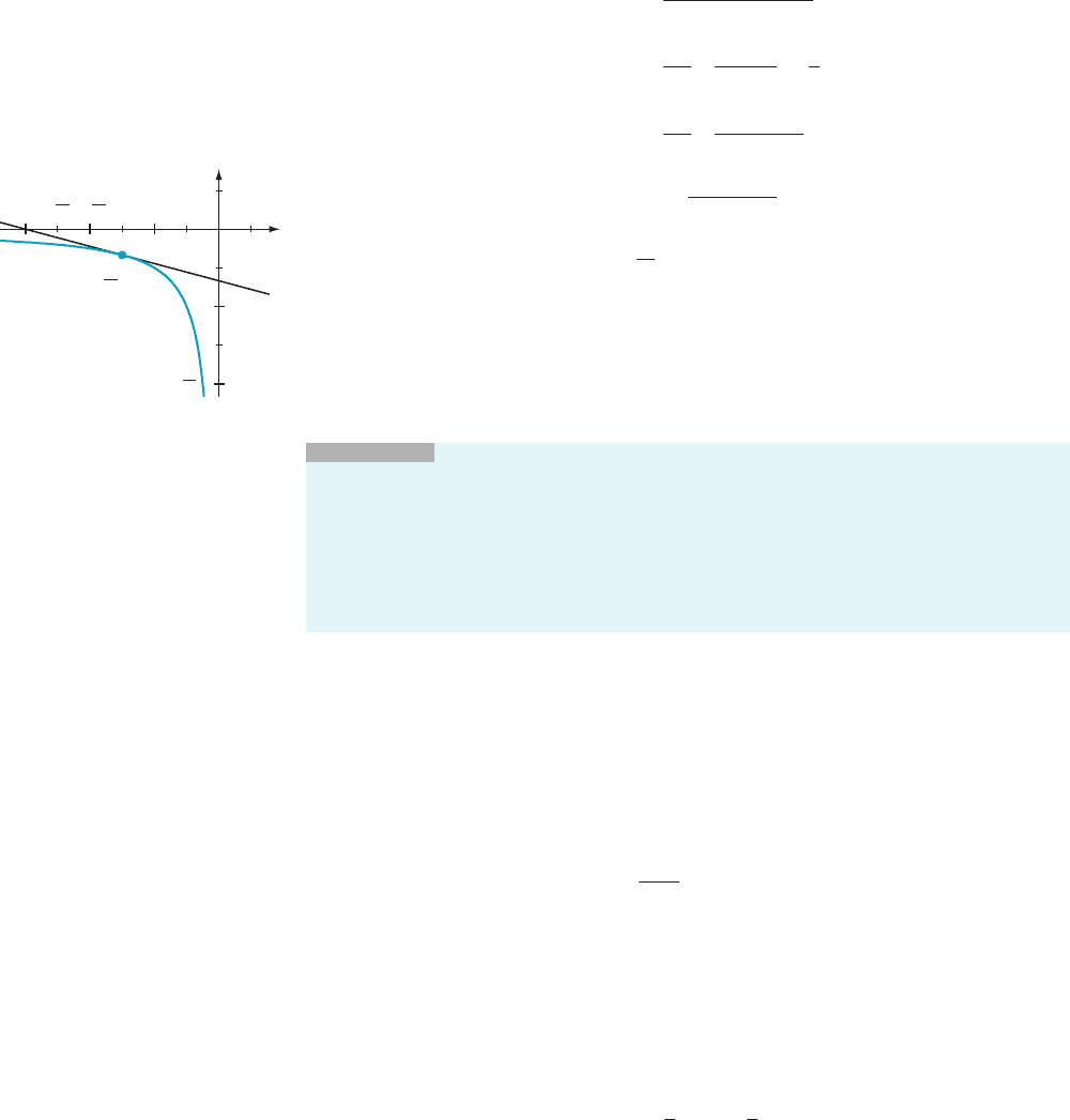
⁄ EXAMPLE 9 Find the tangent line to the curve y 5 1/x at the point P 5

(23, 21/3).

Solution Let f (x) 5 1/x.

Let c 6¼0 be a point in the domain of f. We calculate

ðcÞ 5 lim

Δx-0

f ðc 1 Δ x Þ2 f ðcÞ

Δx

5 lim

Δx-0

Δx



c 1 Δx



5 lim

Δx-0

Δx



2 Δx

cðc 1 Δ x Þ



52 lim

Δx-0

cðc 1 Δ x Þ

Setting c 523, we see that the slope of the tangent line at P is f

ð2 3Þ 5

2 1/(2 3)

521/9. According to deﬁnition (3.1.12), the equation of the tangent line

is y 5 (2 1/9) (x 2 (2 3)) 1 (2 1/3) , or y 52x/9 2 2/3. Figure 9 illustrates the graph

of y 5 1/x and its tangent line at P.

INSIGHT

From the solution to Example 9, we see that f

ðcÞ521=c

if f (x) 5 1/x.

Using equation (3.1.7), we deduce that, if α is a constant and f ðxÞ5 α=x, then

ðcÞ52α=c

. Letting n521, we may restate this result as follows: if f ðxÞ5 α  x

, then

ðcÞ5 α  nc

n21

. In other words, formula (3.1.6), which previously we have shown to hold

for n 5 0, 1, 2, 3, is also true for n 521:

If f ðxÞ5 α  x

for n 521; 0; 1; 2; or 3; then f

ðcÞ5 α nc

n21

ð3:1:13Þ

Normal Lines

to Curves

A line L is said to be perpendicular or normal to a curve y 5 f (x) at a point P 5

(c, f (c)) if L is perpendicular to the tangent line to the curve at the point P. If the

tangent line is the horizontal line y 5 f ( c), then the normal line is the vertical

line x 5 c. If the slope f

reciprocal 2 1/f

ðcÞ is the slope of the normal line (by Theorem 1 of Section 1.3).

Thus, if f

ðcÞ6¼0, then

y 52

ðcÞ

ðx 2 cÞ1 f ðcÞð3:1:14Þ

is the normal line to the graph of f at the point (c, f (c)).

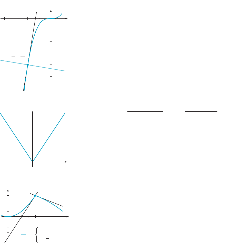
⁄ EX

AMPLE 10 Find the line perpendicular to the curve y 5 x

/2 at the

point P 5 (2 2, 2 4).

Solution Let f (x) 5 x

/2. Using formula (3.1.6) with α 5 1/2 and n 5 3, we have

ðcÞ5

 3c



2

1

2

6

y  

P 



y 



3,



m Figure 9

3.1 Rates of Change and Tangent Lines 173

Therefore f

ð2 2Þ5 3 (2 2)

/2 5 6 is the slope of the tangent line to the graph at P.

The slope of the normal line is the negative reciprocal of this number, or 21/6. The

equation of the normal line to the graph of y 5 x

/2 at P is, by (3.1.14),

y 5 (2 1/6) (x 2 (2 2)) 1 (2 4), or y 52x/6 2 13/3. A sketch is shown in Figure 10.

Corners and Vertical

Tangent Lines

The deﬁnition of the tangent line of f at (c, f (c)) requires the two-sided limit

(3.1.11) for the slope. This limit fails to exist if the one-sided limits

‘

5 lim

Δx-0

f ðc 1 Δ x Þ2 f ðcÞ

Δx

and ‘

5 lim

Δx-0

f ðc 1 Δ x Þ2 f ðc Þ

Δx

exist and are ﬁnite but unequal. In this case, the line y 2 f ðcÞ5 ‘

ðx 2 cÞ is “tan-

gent” to that part of the graph of f to the left of c, and the line y 2 f ðcÞ5 ‘

ðx 2 cÞ is

“tangent” to that part of the graph of f to the right of c. But there is no line that

is tangent to both sides of the graph of f. Therefore f does not have a tangent line

at ðc; f ðcÞÞ. We say that f has a corner at (c, f (c)). A familiar example is the

vee-shaped graph of y 5 jxj, which has a corner at (0, 0): see Figure 11.

⁄ EX

AMPLE 11 Does the graph of the function f deﬁned by

f ðxÞ5

if x , 2

5 2 x

=4ifx $ 2



have a tangent line at the point P 5 (2, 4)?

Solution Notice

that the left and right limits of f (x)atx 5 2 exist and equal 4.

Because these limits exist and agree, f is continuous at 2. For c 5 2, we have

lim

Δx-0

f ðc 1 ΔxÞ2 f ðcÞ

Δx

5 lim

Δx-0



ð21ΔxÞ

2 4



Δx

5 lim

Δx-0

ðΔxÞ

1 4Δx

Δx

5 lim

Δx-0

ð4 1 Δ x Þ

5 4:

On the other hand,

lim

Δx-0

f ðc 1 Δ x Þ2 f ðcÞ

Δx

5 lim

Δx-0



5 2

ð21ΔxÞ





5 2

 2



Δx

5 lim

Δx-0

2 Δx 2

ðΔxÞ

Δx

5 lim

Δx-0



2 1 2

Δx



521:

Because the one-sided limits exist but are unequal, the graph of f has a corner at P.

The graph of f is shown in Figure 12. The lines that are “one-sided” tangents are

included in the plot. The graph does not have a tangent line at P.

y  x

m Figure 11

4

2

4

2

y  6(x  2)  4

6

Tangent line

Normal line

(2, 4)

y 

y   

m Figure 10

4231

2

4

(2, 4)

y 

5 

if x  2

if x  2

m Figure 12

174 Chapter

3 The Derivative