Bird R.B., Stewart W.E., Lightfoot E.N. Transport Phenomena
Подождите немного. Документ загружается.


Questions for Discussion
667
It has been suggested4 that
Eq.
21.5-20
is also true for the micromixing stage. Where this
can be assumed (e.g., in the common situation where macromixing is rate controlling), it
follows that reactive and nonreactive processes lead to identical descriptions of solute
fluctuations.
In practice, fast reactions
(e-g.,
neutralization of acids with bases) are often used to
determine the effectiveness of mixers, as these are much easier to follow experimentally
than nonreactive mixing. Frequently one can use simple macroscopic measures such as
temperature rise or an indicator color change. However, the measurement of concentra-
tion fluctuations can provide more insight into the nature and the course of the mixing
process.
Slow reactions
are also important, and we consider the special case of irreversible sec-
ond-order kinetics, defined by
When this is time-smoothed, we get
We find, therefore, that the fluctuations in solute concentration increase the time-
smoothed reaction rate relative to that when a simple product of time-smoothed concen-
trations is used. It is, however, difficult to assess the practical importance of this effect.
We illustrate this point by a simple order-of-magnitude analysis, beginning with the
definition of a reaction time constant
tA
for one of the reactants, here solute
A:
To a first approximation, we may write
tA
=
l/krcB0
Fast and slow reactions may then be defined as those for which
t,,
>>
tA
fast reaction
t,,
< <
tA
slow reaction
We have already discussed the case of fast reaction. For slow reactions, turbulence has
no significant effect, because fluctuations become negligible before any appreciable reac-
tion has taken place.
If the mixing and reaction time constants are of the same order of magnitude, a
deeper analysis than the above is needed. Such an analysis must include a model for the
turbulent motion, and does not appear to be presently available.
QUESTIONS
FOR
DISCUSSION
1.
Discuss the similarities and differences between turbulent heat and mass transport.
2.
Discuss the behavior of first- and higher-order reactions in the time-smoothing of the equa-
tion of continuity for
a
given species. What are the consequences of this?
3.
To what extent are the turbulent momentum flux, heat flux, and mass flux similar in form?
4.
What empiricisms are available for describing the turbulent mass flux?
5.
How can eddy diffusivities be measured, and on what do they depend?
6.
Would you expect to get trustworthy results for mass transfer in turbulent tube flow without
chemical reaction just by setting
Rx
=
0
in Eq.
21.4-8?
-
-
-
-
K.-T.
Li
and
H.
L.
Toor,
Ind. Eng.
Chem.
Fundam.,
25,719-723
(1986).

668
Chapter 21 Concentration Distributions in Turbulent Flow
PROBLEMS
21~.1.
Determination of eddy diffusivity (Figs. 18C.1 and 21A.1). In Problem 18C.1 we gave the
formula for the concentration profiles in diffusion from a point source in
a
moving stream. In
isotropic highly turbulent flow, Eq. 18C.1-2 may be modified by replacing
9,,
by
the eddy
diffusivity
9zL.
This equation has been found to be useful for determining the eddy
diffusivity. The molar flow rate of carbon dioxide is 1/1000 that of air.
(a) Show that if one plots lnsc, versus
s
-
z
the slope is -vo/29$b.
(b) Use the data on the diffusion of CO, from a point source in a turbulent air stream shown
in Fig. 21A.1 to get
a$),
for these conditions: pipe diameter, 15.24 cm; v,
=
1512 cm/s.
(c)
Compare the value of
9jfL
with the molecular diffusivity
BAB
for the system C02-air.
(d) List all assumptions made
in
the calculations.
Answer:
(b)
9jf',
=
19 cm2/s
Heat and mass transfer analogy. Write the mass transfer analog of Eq. 13.4-19. What are the
limitations of the resulting equation?
Wall mass
flux
for turbulent flow with no chemical reactions. Use the diffusional analog of
Eq. 13.4-20 for turbulent flow in circular tubes, and the Blasius formula for the friction factor,
to obtain the following expression for the Sherwood number,
valid for large Schmidt numbers.'
Alternate expressions for the turbulent mass flux. Seek an asymptotic expression for the
turbulent mass flux for long circular tubes with a boundary condition of constant wall mass
flux. Assume that the net mass transfer across the wall is small.
(a) Parallel the approach to laminar flow heat transfer
in
510.8 to write
in which
6
=
r/D,
5
=
(z/D)/ReSc,
o,,
is the inlet mass fraction of
A,
and
j,,
is the interfacial
mass flux of
A
into the fluid.
Fig.
21A.1. Concentration traverse data for
C02 injected into a turbulent air stream with
Re
=
119,000 in a tube of diameter 15.24 cm.
The circles are concentrations at a distance
z
=
112.5 cm downstream from the injection
point, and the crosses are concentrations at
z
=
152.7 cm. [Experimental data are taken
-0.6 -0.4 -0.2
0
0.2 0.4
0.6
from W.
L.
Towle and
T.
K.
Sherwood,
Ind.
r/R
-
Eng.
Chem., 31,457462 (1939).]
-
'
0.
T.
Hanna,
0.
C.
Sandall,
and
C.
L.
Wilson,
Ind.
Eng.
Chem.
Res.,
28,2286-2290 (1987).

Problems
669
(b)
Next use the equation of continuity for species
A
to obtain
in which Sc"'
=
p'"/p9$~. This equation is to be integrated with the boundary conditions that
II,
is finite at
5
=
0 and
dII,/df
=
-1 at
5
=
i.
(c)
Integrate once with respect to
[
to obtain
dn,
-
t
-
4
It1''
(vz/(vz))[dt
--
-
(21 B.2-3)
d5
f[1
+
(Sc/S~(~')(~'~'/p)l
An asymptotic expression for the turbulent mass flux.' Start with the final result of Problem
21B.2, and note that for sufficiently high Sc all curvature of the concentration profile will take
place very near the wall, where
v,/(v,)
=
0 and
5
=
i.
Assume that Sdt'
=
1
and use Eq. 5.4-2
to obtain
dn,
-
-- -
1
-
-
1
(21B.3-1)
4
[I
+
SC(~'"/~)I 1
+
sc(yv*/14.5~)~
Introduce the new coordinate
77
=
S~"~(yv,/14.5~) into Eq. 21B.3-1 to get an equation for
dII/dv
valid within the laminar sublayer. Then integrate from
q
=
0 (where
w,
=
w,,)
to
77
=
(where
o,
=
w,,)
to obtain an explicit relation for the wall mass
flux
jAO.
Compare with the analog of
Eq. 13.4-20 obtained
in
Problem 21A.2.
Deposition of silver from
a
turbulent stream (Fig. 21B.3). An approximately 0.1
N
solution of
KNO,
containing 1.00
X
lop6
g-equiv. AgNO, per liter is flowing between parallel Ag plates,
-
Movement of electrons
--+
r"
Ag
+
Ag'
+
e-
Anode
4
Cathode
1
4
Fig.
218.3.
(a)
Electrodeposition of Ag' from
a
turbulent stream flowing in the positive
z
direction between two
parallel plates.
(b)
Concentration gradients in electrodeposition of Ag at an electrode.
'
C.
S.
Lin,
R.
W.
Moulton, and
G.
L. Putnam,
Ind.
Eng.
Chem.,
45,636
(1953).

670
Chapter 21 Concentration Distributions in Turbulent Flow
as shown in Fig. 21B.3(a). A small voltage is applied across the plates to produce a deposition
of Ag on the cathode (lower plate) and to polarize the circuit completely (that is, to maintain
the Agt concentration at the cathode very nearly zero). Forced diffusion may be ignored, and
the
Ag+
may be considered to be moving to the cathode by ordinary (that is, Fickian) diffu-
sion and eddy diffusion only. Furthermore, this solution is sufficiently dilute that the effects
of the other ionic species on the diffusion of Agf are negligible.
(a)
Calculate the Ag' concentration profile, assuming that (i) the effective binary diffusivity
of
Ag+
through water is 1.06
X
lop5
cm2/s;
(ii)
the truncated Lin, Moulton, and Putnam ex-
pression of Eq. 5.4-2 for the turbulent velocity distribution in round tubes is valid for "slit
flow" as well, if four times the h draulic radius is substituted for the tube diameter; (iii) the
plates are 1.27 cm apart, and
&
is 11.4 cm/s.
(b)
Estimate the rate of deposition of Ag on the cathode, neglecting all other electrode reactions.
(c)
Does the method of calculation in part (a) predict a discontinuous slope for the concentra-
tion profile at the center plane of the system? Explain.
Answers:
(a)
See Fig. 218.3(b);
(b)
6.7
X
lo-'*
equiv/cm2. s
21B.5.
Mixing-length expression for the velocity profile.
(a)
Start with Eq. 5.5-3, and show that for steadily driven, fully developed turbulent flow in
a tube
(b)
Next set 7,
=
72'
+
72, where
7:)
is given by the cylindrical coordinate analog of Eq.
5.2-9,
and
?:'
by Eq. 5.5-5. Show that Eq. 21B.5-1 then becomes
(c)
Obtain Eq. 21.4-13 from Eq. 21B.5-2 by introducing the dimensionless symbols used in the
former equation.

Chapter
22
Interphase Transport in
Nonisothermal Mixtures
Definition of transfer coefficients in one phase
Analytical expressions for mass transfer coefficients
Correlation of binary transfer coefficients in one phase
Definition of transfer coefficients in two phases
Mass transfer and chemical reactions
Combined heat and mass transfer by free convection
Effects of interfacial forces on heat and mass transfer
Transfer coefficients at high net mass transfer rates
Matrix approximations for multicomponent mass transport
Here we build on earlier discussions of binary diffusion to provide means for predicting
the behavior of mass transfer operations such as distillation, absorption, adsorption, ex-
traction, drying, membrane filtrations, and heterogeneous chemical reactions. This chap-
ter has many features in common with Chapters
6
and
14.
It is particularly closely
related to Chapter 14, because there are many situations where the analogies between
heat and mass transfer can be regarded as exact.
There are, however, important differences between heat and mass transfer, and we
will devote much of this chapter to exploring these differences. Since many mass transfer
operations involve fluid-fluid interfaces, we have to deal with distortions of the interfa-
cial shape by viscous drag and by surface tension gradients resulting from inhomo-
geneities in temperature and composition. In addition, there may be interactions
between heat and mass transfer, and there may be chemical reactions occurring. Further-
more, at high mass transfer rates, the temperature and concentration profiles may be dis-
torted. These effects complicate and sometimes invalidate the neat analogy between heat
and mass transfer that one might otherwise expect.
In Chapter 14 the interphase heat transfer involved the movement of heat to or from
a solid surface, or the heat transfer between two fluids separated by a solid surface. Here
we will encounter heat and mass transfer between two contiguous phases: fluid-fluid or
fluid-solid. This raises the question as to how to account for the resistance to diffusion
provided by the fluids on both sides of the interface.
We begin the chapter by defining, in 522.1, the mass and heat transfer coefficients
for binary mixtures in one phase (liquid or gas). Then in 522.2 we show how analytical
solutions to diffusion problems lead to explicit expressions for mass transfer coefficients.
In that section we give some analytic expressions for mass transfer coefficients at high

672
Chapter
22
Interphase Transport in Nonisothermal Mixtures
Schmidt numbers for a number of relatively simple systems. We emphasize the different
behavior of systems with fluid-fluid and solid-fluid interfaces.
In 522.3 we show how dimensional analysis leads to predictions involving the Sher-
wood number (Sh) and the Schmidt number (Sc), which are the analogs of the Nusselt
number (Nu) and the Prandtl number (Pr) defined in Chapter 14. Here the emphasis is
on the analogies between heat transfer in pure fluids and mass transfer in binary mix-
tures. Then in 522.4 we proceed to the definition of mass transfer coefficients for systems
with diffusion in two adjoining phases. We show there how to apply the information
about mass transfer in single phases to the understanding of mass transfer between two
phases.
Finally, in the last five sections of the chapter, we take up some effects that are pecu-
liar to mass transfer systems: mass transfer with chemical reactions (§22.5), the interac-
tion of heat and mass transfer processes in free convection (§22.6), the complicating
factors of interfacial tension forces and Marangoni effects (522.71, the distortions of tem-
perature and concentration profiles that arise in systems with large net mass transfer
rates across the interface (S22.8); and finally the matrix analysis of mass transport in mul-
ticomponent systems. In this chapter the emphasis is on the non-analogous behavior of
heat and mass transfer systems.
In this chapter we have limited the discussion to a few key topics on mass transfer
and transfer coefficient correlations. Further information is available in specialized text-
books on these and related topics.14
g22.1
DEFINITION OF TRANSFER COEFFICIENTS
IN
ONE PHASE
In this chapter we relate the rates of mass transfer across phase boundaries to the rele-
vant concentration differences, mainly for binary systems. These relations are analogous
to the heat transfer correlations of Chapter 14 and contain
mass
transfer
coeficients
in
place of the heat transfer coefficients of that chapter. The system may have a true phase
boundary, as in Fig. 22.1-1,2, or
4,
or an abrupt change in hydrodynamic properties,
as
in the system of Fig. 22.1-3, containing a porous solid. Figure 22.1-1 shows the evapora-
tion of a volatile liquid, often used in experiments to develop mass transfer correlations.
Figure 22.1-2 shows a permselective membrane, in which a selectively permeable sur-
face permits more effective transport of solvent than of a solute that is to be retained, as
in ultrafiltration of protein solutions and the desalting of sea water. Figure 22.1-3 shows
a macroscopically porous solid, which can serve as a mass transfer surface or can
pro-
vide sites for adsorption or reaction. Figure 22.1-4 shows an idealized liquid-vapor con-
tactor where the mass transfer interface may be distorted by viscous or surface-tension
forces.
Stream of gas
B
h
t
Vapor
A
moving
into gas stream
Fig.
22.1-1.
Example of
Interface
+
mass transfer across a
plane boundary: drying
of
a
saturated slab.
'
T.
K.
Sherwood,
R.
L.
Pigford, and
C.
R.
Wilke,
Mass Transfer,
McGraw-Hill, New York (1975).
R.
E.
Treybal,
Mass Transfer Operations,
3rd edition, McGraw-Hill, New York (1980).
%.
L.
Cussler,
Diffusion: Mass Transfer in
Fluid
Systems,
2nd edition, Cambridge University Press
(1997).
9.
E.
Rosner,
Transport Processes in Chemically Reacting Flow Systems
(Unabridged), Dover, New
York (2000).

$22.1
Definition of Transfer Coefficients in One Phase
673
Representative Membrane Processes
Pek
1:
Dialysis
Blood oxygenation
re'>>
1:
Microfiltration
Ultrafiltration
Nanofiltration
Reverse osmosis
Membrane
4
Fig.
22.1-2.
Two rather typical kinds of membrane separators,
classified here according to a Peclet number, P6
=
6v/geff, for
the flow through the membrane. Here
6
is the membrane
thickness,
v
is the velocity at which solvent passes through
the membrane, and
'&
is the effective solute diffusivity
through the membrane. The heavy line represents the mem-
brane, and the arrows represent the flow along or through the
membrane.
Stream of hot gas
A
Injected gas
A
moving
/
away from wall
Cold gas
A
pumped
through wall
Upward-
-
moving gas
At interface
r=R
y
=
0
and
=
N~O
NB
=
NBO
Fig.
22.1-3.
Example of
mass transfer through a
porous wall: transpira-
tion cooling.
Tube wall
Fig.
22.1-4.
Example of a gas-liquid con-
tacting device: the wetted-wall column.
Two chemical species
A
and
B
are mov-
ing from the downward-flowing liquid
stream into the upward-flowing gas
stream in a cylindrical tube.
674
Chapter 22 Interphase Transport in Nonisothermal Mixtures
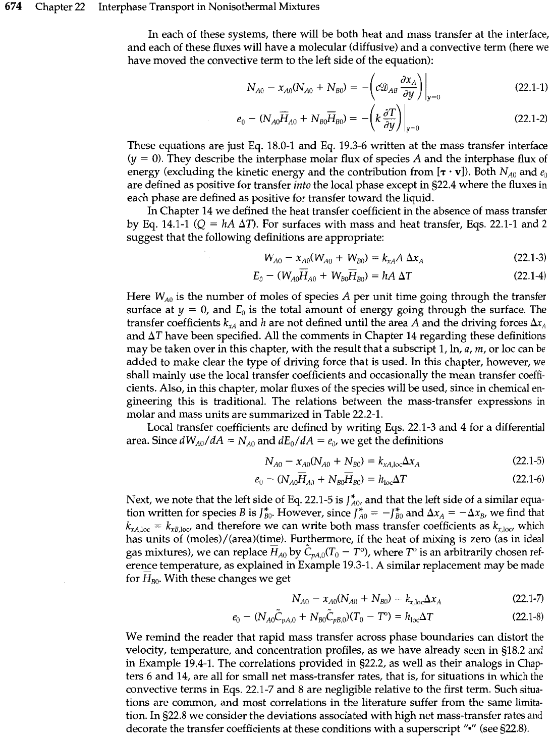
In each of these systems, there will be both heat and mass transfer at the interface,
and each of these fluxes will have a molecular (diffusive) and a convective term (here we
have moved the convective term to the left side of the equation):
These equations are just Eq. 18.0-1 and Eq. 19.3-6 written at the mass transfer interface
(y
=
0). They describe the interphase molar flux of species A and the interphase flux of
energy (excluding the kinetic energy and the contribution from
[T
.
vl).
Both NAo and
e,
are defined as positive for transfer
into
the local phase except
in
522.4 where the fluxes
in
each phase are defined as positive for transfer toward the liquid.
In Chapter
14
we defined the heat transfer coefficient in the absence of mass transfer
by Eq. 14.1-1
(Q
=
hA AT). For surfaces with mass and heat transfer, Eqs. 22.1-1 and
2
suggest that the following definitions are appropriate:
Here WAo is the number of moles of species A per unit time going through the transfer
surface at
y
=
0, and
E,
is the total amount of energy going through the surface. The
transfer coefficients
kxA
and
h
are not defined until the area A and the driving forces
Ax,
and AT have been specified. All the comments in Chapter 14 regarding these definitions
may be taken over in this chapter, with the result that a subscript 1, In,
a,
m,
or loc can
be
added to make clear the type of driving force that is used. In this chapter, however,
we
shall mainly use the local transfer coefficients and occasionally the mean transfer coeffi-
cients. Also, in this chapter, molar fluxes of the species will be used, since in chemical en-
gineering this is traditional. The relations between the mass-transfer expressions
in
molar and mass units are summarized in Table 22.2-1.
Local transfer coefficients are defined by writing Eqs. 22.1-3 and 4 for a differential
area. Since d WA,/dA
=
NAO and dE,/dA
=
e,,
we get the definitions
Next, we note that the left side of Eq. 22.1-5 is
J;,,
and that the left side of a similar equa-
tion written for species
B
is
J&.
However, since
J;,
=
-J&
and
AX,
=
-AxB, we find that
kxA,loc
=
kxB,loc,
and therefore we can write both mass transfer coefficients as
kx,lOc,
which
has units of (moles)/(area)(time).
-
Furthermore, if the heat of mixing is zero (as in ideal
gas mixtures), we can replace HA, by (?,,,(T,
-
To), where To is an arbitrarily chosen ref-
erence temperature, as explained in Example 19.3-1.
A
similar replacement may be made
for &,. With these changes we get
We remind the reader that rapid mass transfer across phase boundaries can distort the
velocity, temperature, and concentration profiles, as we have already seen in 518.2 and
in Example 19.4-1. The correlations provided in s22.2, as well as their analogs in Chap-
ters 6 and 14, are all for small net mass-transfer rates, that is, for situations in which
the
convective terms in Eqs. 22.1-7 and 8 are negligible relative to the first term. Such situa-
tions are common, and most correlations in the literature suffer from the same limita-
tion. In 522.8 we consider the deviations associated with high net mass-transfer rates and
decorate the transfer coefficients at these conditions with a superscript
"*"
(see 522.8).

6j22.1
Definition of Transfer Coefficients in One Phase
675
In much of the chemical engineering literature, the mass transfer coefficients are de-
fined by
The relation of this "apparent" mass transfer coefficient to that defined by
Eq.
22.1-7 is
in which r
=
NBo/NAo. Other widely used mass transfer coefficients are defined by
for liquids and
for gases. In the limit of low solute concentrations and low net mass transfer rates, for
which most correlations have been obtained,
The superscript
0
indicates that these quantities are applicable only for small mass-trans-
fer rates and small
mole
fractions of species
A.
In many industrial contactors, the true interfacial area is not known. An example of
such a system would be a column containing a random packing of irregular solid parti-
cles. In such a situation, one can define a volumetric mass transfer coefficient,
kg,
incor-
porating the interfacial area for a differential region of the column. The rate at which
moles of species
A
are transferred to the interstitial fluid in a volume
Sdz
of the column is
then given by
Here the interfacial area, a, per unit volume is combined with the mass transfer coeffi-
cient,
S
is the total column cross section, and
z
is measured in the primary flow direction.
Correlations for predicting values of these coefficients are available, but they should be
used with caution. Rarely do they include all the important parameters, and as a result
they cannot be safely extrapolated to new systems. Furthermore, although they are usu-
ally described as "local," they actually represent a poorly defined average over a wide
range of interfacial
We conclude this section by defining a dimensionless group widely used in the
mass-transfer literature and in the remainder of this book:
which is called the Sherwood number based on the characteristic length lo. This quantity
can be "decorated with subscripts
1,
a, m, In, and loc in the same manner as
h.
'
J.
Stichlmair and
J.
F.
Fair,
Distillation Principles and Practice,
Wiley, New York (1998).
H.
Z.
Kister,
Distillation Design,
McGraw-Hill, New York (1992).
J.
C.
Godfrey and
M.
M.
Slater,
Liquid-Liquid Extraction Equipment,
Wiley, New York (1994).
".
H.
Perry and
D.
W. Green,
Chemical Engineers' Handbook,
8th edition, McGraw-Hill, New York
(1997).
J.
E.
Vivian and
C.
J.
King,
in
Modem Chemical Engineering
(A.
Acrivos,
ed.),
Reinhold, New York (1963).

676
Chapter
22
Interphase Transport in Nonisothermal Mixtures
522.2
ANALYTICAL EXPRESSIONS FOR
MASS TRANSFER COEFFICIENTS
In the preceding chapters we obtained a number of analytical solutions for concentra-
tion profiles and for the associated molar fluxes. From these solutions we can now derive
the corresponding mass transfer coefficients. These are usually presented in dimensionless
form in terms of Sherwood numbers. We summarize these analytical expressions here for
use in later sections of this chapter. All of the results given in this section are for systems
with a slightly soluble component
A,
small diffusivities %AB, and small net mass-transfer
rates, as defined in 9322.1 and 8. It may be helpful at this point to refer to Table 22.2-1,
where the dimensionless groups for heat and mass transfer have been summarized.
Mass Transfer in Falling Films on Plane Surfaces
For the absorption of a slightly soluble gas
A
into a falling film of pure liquid
B,
we can
put the result of Eq. 18.5-18 into the form of Eq. 22.1-3 (appropriately modified for molar
concentration units in the manner of
Eq.
22.1-ll), thus
Table
22.2-1
Analogies Among Heat and Mass Transfer at Low Mass-Transfer Rates
Heat transfer
Binary mass transfer Binary mass transfer
quantities
quantities (isothermal quantities (isothermal
(pure fluids)
fluids, molar units) fluids, mass units)
Profiles
T
*A
w
A
Diffusivity
a
=
k/pCp
9
AB
9
AB
Effect of profiles
on density
Transfer coefficient
Q
h=-
A
AT
Dimensionless groups
Re
=
I,v,p/p
Re
=
l,v@/p
common to all three Fr
=
v;/gl,
Fr
=
v;/gl,
correlations
Dimensionless groups
Nu
=
hlO/k
Sh
=
kxlO/&dAB
Sh
=
~,~O/P~AB
that are different
~r
=
&p/k
Sc
=
p/pgAB
Sc
=
p/pEbAB
Gr
=
l&2gpAT/p2
Gr,
=
I&2g5A~A/p2
Gr,
=
l~p2g[Aw,/p2
P6
=
RePr
=
l,v,~,/k
P6
=
ReSc
=
IOvo/9AB
P6
=
ReSc
=
I,v,,/~~,
Notes:
(a) The subscript
0
on
I,
and
v,
indicates the characteristic length and velocity respectively, whereas the subscript
0
on the mole
(or mass) fraction and molar (or mass) flux means "evaluated at the interface." (b)
All
three of these Grashof numbers can be written as
Gr
=
lipg
AplP2,
provided that the density change is caused only by a difference of temperature or composition.