Bichop R.H. (Ed.) Mechatronic Systems, Sensors, and Actuators: Fundamentals and Modeling

Подождите немного. Документ загружается.

20-14 Mechatronic Systems, Sensors, and Actuators

The governing equations of these motions are as follows:

Rectilinear acceleration (20.1)

Angular acceleration (20.2)

Curvilinear acceleration (20.3)

where a and

are the accelerations; v and

are the speeds; s is the distance;

is the angle; i, j, and k

are the unit vectors in x, y, and z directions, respectively.

For the correct applications of the accelerometers, a sound understanding of the characteristics of the

motion under investigation is very important. The application areas may be linear and vibratory motion,

angular motion, monitoring of the tilt of an object, or various forms of combinations. In each case, the

correct selection and mounting of the accelerometer is necessary.

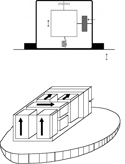
The majority of accelerometers can be viewed and analyzed as a single-degree-of-freedom seismic

instrument that can be characterized by a mass, a spring, and a damper arrangement as shown in

Figure 20.18. In the case of multi-degrees-of-freedom systems, the principles of curvilinear motion can

be applied as in Equation 20.3 and multiple transducers must be used to create uniaxial, biaxial, or triaxial

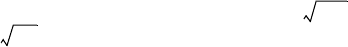
sensing points of the measurements. A typical example is the inertial navigation and guidance systems

as illustrated in Figure 20.20. In such applications, acceleration sensors play an important role in orien-

tation and direction finding. Usually, miniature triaxial sensors detect changes in roll, pitch, and azimuth

in x, y, and z directions.

FIGURE 20.18 A typical seismic accelerometer.

FIGURE 20.19 Arrangements of accelerometers in navigation and guidance systems.

Seismic mass

Housing

(t)

Spring

Damper

Displacement

transducer

Work piece

sin

Computer and

signal processing

Gyro Y

Accel Y

Gyro X

Accel X

Gyro Z

Accel Z

∆v

∆t

------

∆t→0

lim

-----

dds/dt()

--------------------

-------

=== =

∆

∆t

--------

∆t→0

lim

-------

/dt()

----------------------

--------

=== =

-----

--------

-------

k++==

9258_C020.fm Page 14 Tuesday, October 9, 2007 9:08 PM

Sensors 20-15

If a single-degree-of-freedom system behaves linearly in a time invariant manner, the basic second-

order differential equation describing the motion of the forced mass–spring system can be written as

(20.4)

where f(t) is the force, m is the mass, c is the velocity constant, and k is the spring constant.

Nevertheless, the base of the accelerometer is in motion too. When the base is in motion, the force is

transmitted through the spring to the suspended mass, depending on the transmissibility of the force to

the mass. Equation 20.4 may be generalized by taking the effect motion of the base into account as

(20.5)

where z = x

– x

is the relative motion between the mass and the base, x

is the displacement of the base,

is the displacement of mass, and

is the angle between the sense axis and gravity.

The complete solution to Equation 20.5 can be obtained by applying the superposition principle. The

sup-erposition principle states that if there are simultaneously superimposed actions on a body, the total

effect can be obtained by summing the effects of each individual action. Using superposition and using

Laplace transforms gives

(20.6)

(20.7)

where s is the Laplace operator, K = 1/k is the static sensitivity,

= is the undamped critical

frequency (rad/s), and

= (c/2) is the damping ratio.

As can be seen in the performance of accelerometers, the important parameters are the static sensitivity,

the natural frequency, and the damping ratio, which are all functions of mass, velocity, and spring

constants. Accelerometers are designed and manufactured to have different characteristics by suitable

selection of these parameters. A short list of major manufacturers is given in Table 20.1.

20.2.3 Vibrations

This section is concerned with applications of accelerometers to measure physical properties such as

acceleration, vibration and shock, and the motion in general. Although there may be fundamental

differences in the types of motions, a sound understanding of the basic principles of the vibration will

lead to the applications of accelerometers in different situations by making appropriate corrective

measures.

Vibration is an oscillatory motion resulting from application of varying forces to a structure. The

vibrations can be periodic, stationary random, nonstationary random, or transient.

20.2.3.1 Periodic Vibrations

In periodic vibrations, the motion of an object repeats itself in an oscillatory manner. This can be

represented by a sinusoidal waveform

(20.8)

ft() m

--------

------

kx++=

-------

-----

kz++ mg

----------

–cos=

Xs()

Fs()

----------

--------

cs k++=

Xs()

Fs()

----------

1++

---------------------------------------------

k/m

xt() X

t()sin=

9258_C020.fm Page 15 Tuesday, October 9, 2007 9:08 PM

20-16 Mechatronic Systems, Sensors, and Actuators

where x(t) is the time-dependent displacement,

= 2

ft is the angular frequency, and X

is the maximum

displacement from a reference point.

The velocity of the object is the time rate of change of displacement,

(20.9)

where v(t) is the time-dependent velocity, and V

is the maximum velocity.

The acceleration of the object is the time rate of change of velocity,

(20.10)

where a(t) is the time-dependent acceleration, and A

is the maximum acceleration.

TABLE 20 .1 List of Manufacturers

Analog Devices, Inc. Kistler Instrument Corp.

1 Technology Way, P.O. Box 9106 75 John Glenn Dr.

Norwood, MA 02062-9106 USA Amherst, NY 14228 2119 USA

Tel: 781-329-4700 Tel: 888-KISTLER (547-8537)

Fax: 781-326-8703 Fax: 716-691-5226

Aydin Telemetry Oceana Sensor Technologies, Inc.

47 Friends Lane & Penns Trail 1632-T Corporate Landing Pkwy.

Newtown, PA 18940 0328 USA Virginia Beach, VA 23454 USA

Tel: 215-968-4271 Tel: 757-426-3678

Fax: 215-968-3214 Fax: 757-426-3633

Bruel & Kjaer PCB Piezotronics, Inc.

2815-A Colonnades Court 3425-T Walden Ave.

Norcross, GA 30071 USA Depew, NY 14043 2495 USA

Tel: 800-332-2040 Tel: 716-684-0001

Fax: 770-447-8440 Fax: 716-684-0987

Dytran Instruments, Inc. Piezo Systems, Inc.

21592 Marilla St. 186 Massachusetts Ave.

Chatsworth, CA 91311 USA Cambridge, MA 02139-4229 USA

Tel: 800-899-7818 Tel: 617-547-1777

Fax: 800-899-7088 Fax: 617-354-2200

Endevco Corp. Rieker Instrument Co.

30700 Rancho Viejo Rd. P.O. Box 128

San Juan Capistrano, CA 92675 USA Folcroft, PA 19032 0128 USA

Tel: 800-982-6732 Tel: 610-534-9000

Fax: 949-661-7231 Fax: 610-534-4670

Entran Devices, Inc. Sensotec, Inc.

10-T Washington Ave. 2080 Arlingate Lane

Fairfield, NJ 07004 USA Columbus, OH 43228 USA

Tel: 888-8-ENTRAN (836-8726) Tel: 800-858-6184

Fax: 973-227-6865 Fax: 614-850-1111

GS Sensors, Inc. Techkor Instrumentation

16 W. Chestnut St. 2001 Fulling Mill Rd.

Ephrata, PA 17522 USA P.O. Box 70 Dept. T-1

Tel: 717-721-9727 New Cumberland, PA 17057-0070 USA

Fax: 717-721-9859 Tel: 800-697-4567

Fax: 717-939-7170

vt()

------

t()cos V

/2+()sin== =

at()

-----

--------

−

t()sin A

+()sin== = =

9258_C020.fm Page 16 Tuesday, October 9, 2007 9:08 PM

Sensors 20-17

From the preceding equations it can be seen that the basic form and the period of vibration remains

the same in acceleration, velocity, and displacement. But velocity leads displacement by a phase angle of

90° and acceleration leads velocity by another 90°.

In nature, vibrations can be periodic, but not necessarily sinusoidal. If they are periodic but nonsinu-

soidal, they can be expressed as a combination of a number of pure sinusoidal curves, determined by

Fourier analysis as

(20.11)

where

,…,

are the frequencies (rad/s), X

, X

,…, X

are the maximum amplitudes of respective

frequencies, and

,…,

are the phase angles.

The number of terms may be infinite, and the higher the number of elements, the better the approx-

imation. These elements constitute the frequency spectrum. The vibrations can be represented in the

time domain or frequency domain, both of which are extremely useful in analysis.

20.2.3.2 Stationary Random Vibrations

Random vibrations are often met in nature, where they constitute irregular cycles of motion that never

repeat themselves exactly. Theoretically, an infinitely long time record is necessary to obtain a complete

description of these vibrations. However, statistical methods and probability theory can be used for the

analysis by taking representative samples. Mathematical tools such as probability distributions, probability

densities, frequency spectra, cross-correlations, auto-correlations, digital Fourier transforms (DFTs), fast

Fourier transforms (FFTs), auto-spectral-analysis, root mean squared (rms) values, and digital filter analysis

are some of the techniques that can be employed.

20.2.3.3 Nonstationary Random Vibrations

In this case, the statistical properties of vibrations vary in time. Methods such as time averaging and

other statistical techniques can be employed.

20.2.3.4 Transients and Shocks

Often, short duration and sudden occurrence vibrations need to be measured. Shock and transient

vibrations may be described in terms of force, acceleration, velocity, or displacement. As in the case of

random transients and shocks, statistical methods and Fourier transforms are used in the analysis.

20.2.4 Typical Error Sources and Error Modeling

Acceleration measurement errors occur due to four primary reasons: sensors, acquisition electronics,

signal processing, and application specific errors. In the direct acceleration measurements, the main error

sources are the sensors and data acquisition electronics. These errors will be discussed in the biasing

section and in some cases, sensor and acquisition electronic errors may be as high as 5%. Apart from

these errors, sampling and A/D converters introduce the usual errors, which are inherent in them and

exist in all computerized data acquisition systems. However, the errors may be minimized by the careful

selection of multiplexers, sample-and-hold circuits, and A/D converters.

When direct measurements are made, ultimate care must be exercised for the selection of the correct

accelerometer to meet the requirements of a particular application. In order to reduce the errors, once

the characteristics of the motion are studied, the following particulars of the accelerometers need to be

considered: the transient response or cross-axis sensitivity; frequency range; sensitivity, mass and dynamic

range; cross-axis response; and environmental conditions, such as temperature, cable noise, stability of

bias, scale factor, and misalignment, etc.

20.2.4.1 Sensitivity of Accelerometers

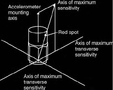
During measurements, the transverse motions of the system affect most accelerometers and the sensitivity

to these motions plays a major role in the accuracy of the measurement. The transverse, also known as

cross-axis, sensitivity of an accelerometer is its response to acceleration in a plane perpendicular to the

xt() X

t Φ

+()X

t Φ

+()

…

t Φ

+()sin++sin+sin+=

9258_C020.fm Page 17 Tuesday, October 9, 2007 9:08 PM

20-18 Mechatronic Systems, Sensors, and Actuators

main accelerometer axis as shown in Figure 20.20. The cross-axis sensitivity is normally expressed as a

percentage of the main-axis sensitivity and should be as low as possible. The manufacturers usually supply

the direction of minimum sensitivity.

The measurement of the maximum cross-axis sensitivity is part of the individual calibration process

and should always be less than 3% or 4%. If high levels of transverse vibration are present, this may

result in erroneous overall results. In this case, separate arrangements should be made to establish the

level and frequency contents of the cross-axis motions. The cross-axis sensitivity of typical accelerom-

eters mentioned in the relevant sections were 2–3% for piezoelectric types and less than 1% for most

others.

20.2.4.2 The Frequency Range

Acceleration measurements are normally confined to using the linear portion of the response curve of

the accelerometer. The response is limited at the low frequencies as well as at the high frequencies by the

natural resonances. As a rule of thumb, the upper-frequency limit for the measurement can be set to

one-third of the accelerometer’s resonance frequency such that the vibrations measured will be less than

1 dB in linearity. It should be noted that an accelerometer’s useful frequency range may be significantly

higher; that is, one-half or two-thirds of its resonant frequency. The measurement frequencies may be

set to higher values in applications in which lower linearity (say 3 dB) is acceptable. The lower measuring

frequency limit is determined by two factors. The first is the low-frequency cutoff of the associated

preamplifiers. The second is the effect of ambient temperature fluctuations to which the accelerometer

may be sensitive.

20.2.4.3 The Mass of Accelerometer and Dynamic Range

Ideally, the higher the transducer sensitivity, the better. Compromises may have to be made for sensitivity

versus frequency, range, overload capacity, size, and so on.

In some cases, high errors will be introduced due to wrong selection of the sensor that is suitable for

a specific application. For example, accelerometer mass becomes important when using small and light

test objects. The accelerometer should not load the structural member, since additional mass can signif-

icantly change the levels and frequency presence at measuring points and invalidate the results. As a

general rule, the accelerometer mass should not be greater than one-tenth the effective mass of the part

or the structure that it is mounted onto for measurements.

The dynamic range of the accelerometer should match the high or low acceleration levels of the

measured objects. General-purpose accelerometers can be linear from 5000g to 10,000g, which is well in

the range of most mechanical shocks. Special accelerometers can measure up to 100,000g.

FIGURE 20.20 Illustration of cross-axis sensitivity.

9258_C020.fm Page 18 Tuesday, October 9, 2007 9:08 PM

Sensors 20-19

20.2.4.4 The Transient Response

Shocks are characterized as sudden releases of energy in the form of short-duration pulses exhibiting

various shapes and rise times. They have high magnitudes and wide frequency contents. In applications

where transient and shock measurements are involved, the overall linearity of the measuring system may

be limited to high and low frequencies by a phenomena known as zero shift and ringing, respectively.

The zero shift is caused by both the phase nonlinearity in the preamplifiers and the accelerometer not

returning to steady-state operation conditions after being subjected to high shocks. Ringing is caused by

high-frequency components of the excitation near-resonance frequency, preventing the accelerometer

from returning back to its steady-state operation condition. To avoid measuring errors due to these

effects, the operational frequency of the measuring system should be limited to the linear range.

20.2.4.5 Full Scale Range and Overload Capability

Most accelerometers are able to measure acceleration in both positive and negative directions. They are

also designed to be able to accommodate overload capacity. Manufacturers also supply information on

these two characteristics.

20.2.4.6 Environmental Conditions

In selection and implementation of accelerometers, environmental conditions such as temperature ranges,

temperature transients, cable noise, magnetic field effects, humidity, and acoustic noise need to be con-

sidered. Manufacturers supply information on environmental conditions.

20.2.5 Inertial Accelerometers

Inertial accelerometers are mechanical accelerometers that make use of a seismic mass that is suspended

by a spring or a lever inside a rigid frame as shown in Figure 20.17. The frame carrying the seismic mass

is connected firmly to the vibrating source whose characteristics are to be measured. As the system

vibrates, the mass tends to remain fixed in its position so that the motion can be registered as a relative

displacement between the mass and the frame. An appropriate transducer senses this displacement and

the output signal is processed further. The displacement sensing element can be made from a variety of

materials exhibiting resistive, capacitive, inductive, piezoelectric, piezoresistive, and optical capabilities.

In practice, the seismic mass does not remain absolutely steady, but it can satisfactorily act as a reference

position for selected frequencies.

By proper selection of mass, spring, and damper combinations, the seismic instrument may be used

for either acceleration or displacement measurements. In general, a large mass and soft spring are suitable

for vibration and displacement measurement, while a relatively small mass and a stiff spring are used in

accelerometers. However, the term seismic is commonly applied to instruments, which sense very low

levels of vibration in the ground or structures.

In order to describe the response of the seismic accelerometer in Figure 20.17, Newton’s second law,

the equation of motion, may be written as

(20.12)

where x

is the displacement of the vibration frame, x

is the displacement of the seismic mass, c is the

velocity constant,

is the angle between the sense axis and gravity, and k is the spring constant.

Ta kin g md

/dt

from both sides of the equation and rearranging gives

(20.13)

where z = x

− x

is the relative motion between the mass and the base.

----------

--------

++ c

--------

()cos++=

-------

-----

kz++ mg

() m

----------

–cos=

9258_C020.fm Page 19 Tuesday, October 9, 2007 9:08 PM

20-20 Mechatronic Systems, Sensors, and Actuators

In Equation 20.12, it is assumed that the damping force on the seismic mass is proportional to velocity

only. If a harmonic vibratory motion is impressed on the instrument such that

(20.14)

where

is the frequency of vibration (rad/s), writing

modifies Equation 20.13 as

(20.15)

where a

= mX

Equation 20.15 will have transient and steady-state solutions. The steady-state solution of the differ-

ential equation 20.15 may be determined as

(20.16)

Rearranging Equation 20.16 results in

(20.17)

where

(= ) is the natural frequency of the seismic mass, (=c/2 ) is the damping ratio.

The damping ratio can be written in terms of the critical damping ratio as = c/c

, where c

= 2,

(= tan

−1

/(k − m )]) is the phase angle, and r (=

) is the frequency ratio.

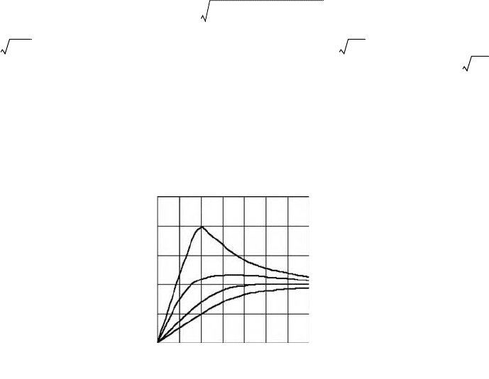
A plot of Equation 20.17 (

−

)

against frequency ratio

, is illustrated in Figure 20.21. This

figure shows that the output amplitude is equal to the input amplitude when

0.7 and

2. The

output becomes essentially a linear function of the input at high frequency ratios. For satisfactory system

performance, the instrument constant

and

should be carefully calculated or obtained from calibrations.

FIGURE 20.21 Frequency versus amplitude ratio of seismic accelerometers.

t() X

t()sin=

−m

----------

tsin=

-------

-----

kz++ mg

() ma

tsin+cos=

()cos

------------------------

tsin

+–()

-----------------------------------------

()cos

------------------------

–()sin

1 r

–()

r()

----------------------------------------------------

k/m

1.0

0.5

0.7

0.25

2.0

3.0

Amplitude ratio

Frequency ratio

________

–x

)

___

9258_C020.fm Page 20 Tuesday, October 9, 2007 9:08 PM

Sensors 20-21

In this way the anticipated accuracy of measurement may be predicted for frequencies of interest. A com-

prehensive treatment of the analysis has been performed by McConnell [7]; interested readers should refer

to this text for further details.

Seismic instruments are constructed in a variety of ways. In a potentiometric instrument, a voltage

divider potentiometer is used for sensing the relative displacement between the frame and the seismic

mass. In the majority of potentiometric accelerometers, the device is filled with a viscous liquid that

interacts continuously with the frame and the seismic mass to provide damping. These accelerometers

have a low frequency of operation (less than 100 Hz) and are mainly intended for slowly varying

accelerations, and low-frequency vibrations. A typical family of such instruments offers many different

models, covering the range of ±1g to ±50g full scale. The natural frequency ranges from 12 to 89 Hz, and

the damping ratio

can be kept between 0.5 and 0.8 by using a temperature compensated liquid-damping

arrangement. Potentiometer resistance may be selected in the range of 1000–10,000 Ω, with a correspond-

ing resolution of 0.45–0.25% of full scale. The cross-axis sensitivity is less than ±1%. The overall accuracy

is ±1% of full scale or less at room temperatures. The size is about 50 mm

with a total mass of about 1/2 kg.

Linear variable differential transformers (LVDTs) offer another convenient means of measurement of

the relative displacement between the seismic mass and the accelerometer housing. These devices have

higher natural frequencies than potentiometer devices, up to 300 Hz. Since the LVDT has lower resistance

to motion, it offers much better resolution. A typical family of liquid-damped differential-transformer

accelerometers exhibits the following characteristics. The full scale ranges from ±2g to ±700g, the natural

frequency from 35 to 620 Hz, the nonlinearity 1% of full scale. The full-scale output is about 1 V with

an LVDT excitation of 10 V at 2000 Hz, the damping ratio ranges from 0.6 to 0.7, the residual voltage

at the null position is less than 1%, and the hysteresis is less than 1% of full scale. The size is about

50 mm

with a mass of about 120 g.

Electrical resistance strain gages are also used for displacement sensing of the seismic mass. In this

case, the seismic mass is mounted on a cantilever beam rather than on springs. Resistance strain gauges

are bonded on each side of the beam to sense the strain in the beam resulting from the vibrational

displacement of the mass. A viscous liquid that entirely fills the housing provides damping of the system.

The output of the strain gauges is connected to an appropriate bridge circuit. The natural frequency of

such a system is about 300 Hz. The low natural frequency is due to the need for a sufficiently large

cantilever beam to accommodate the mounting of the strain gauges.

One serious drawback of the seismic instruments is temperature effects requiring additional compen-

sation circuits. The damping of the instrument may also be affected by changes in the viscosity of the

fluid due to temperature. For instance, the viscosity of silicone oil, often used in these instruments, is

strongly dependent on temperature.

20.2.5.1 Suspended-Mass, Cantilever, and Pendulum-Type Inertial Accelerometers

There are a number of different inertial-type accelerometers, most of which are in development stages

or used under very special circumstances, such as gyropendulum, reaction-rotor, vibrating-string, and

centrifugal-force-balance.

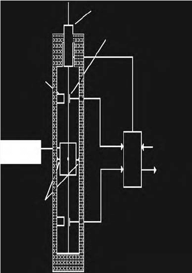
The vibrating-string instrument, Figure 20.22, makes use of a proof mass supported longitudinally by

a pair of tensioned, transversely vibrating strings with uniform cross section and equal lengths and masses.

The frequency of vibration of the strings is set to several thousand cycles per second. The proof mass is

supported radially in such a way that the acceleration normal to the strings does not affect the string

tension. In the presence of acceleration along the sensing axis, a deferential tension exists on the two

strings, thus altering the frequency of vibration. From the second law of motion the frequencies may be

written as

(20.18)

where T is the tension, m

are the mass, and l is the lengths of strings.

-----------

and f

-----------

9258_C020.fm Page 21 Tuesday, October 9, 2007 9:08 PM

20-22 Mechatronic Systems, Sensors, and Actuators

The quantity T

− T

is proportional to ma where a is the acceleration along the axis of the strings.

An expression for the difference of the frequency-squared terms may be written as

(20.19)

Hence

(20.20)

The sum of frequencies ( f

+ f

) can be held constant by serving the tension in the strings with reference

to the frequency of a standard oscillator. Then, the difference between the frequencies becomes linearly

proportional to acceleration. In some versions, the beamlike property of the vibratory elements is used

by gripping them at nodal points corresponding to the fundamental mode of the vibration of the beam,

and at the respective centers of percussion of the common proof mass. The output frequency is propor-

tional to acceleration and the velocity is proportional to phase, thus offering an important advantage.

The improved versions of these devices lead to cantilever-type accelerometers, discussed next.

In a cantilever-type accelerometer, a small cantilever beam mounted on the block is placed against the

vibrating surface, and an appropriate mechanism is provided for varying the beam length. The beam

length is adjusted such that its natural frequency is equal to the frequency of the vibrating surface, and

hence the resonance condition is obtained. Recently, slight variations of cantilever-beam arrangements

are finding new applications in microaccelerometers.

In a different type of suspended-mass configuration, a pendulum is used that is pivoted to a shaft

rotating about a vertical axis. Pickoff mechanisms are provided for the pendulum and the shaft speed.

FIGURE 20.22 A typical suspended-mass vibrating-string accelerometer.

Seismic

mass

Ligaments for

radial support

(to computer)

Standard

frequency

Vibration pickup

String

driver

Tension adjuster

(to constant f

+ f

)

Acceleration

sensing axis

– f

–

-----------------

-----------

–

+()

-----------------------------

9258_C020.fm Page 22 Tuesday, October 9, 2007 9:08 PM

Sensors 20-23

The system is servo controlled to maintain it at null position. Gravitational acceleration is balanced by

the centrifugal acceleration. The shaft speed is proportional to the square root of the local value of the

acceleration.

20.2.6 Electromechanical Accelerometers

Electromechanical accelerometers, essentially servo or null-balance types, rely on the principle of feed-

back. In these instruments, an acceleration-sensitive mass is kept very close to a neutral position or zero

displacement point by sensing the displacement and feeding back the effect of this displacement.

A proportional magnetic force is generated to oppose the motion of the mass displaced from the neutral

position, thus restoring this position just as a mechanical spring in a conventional accelerometer would

do. The advantages of this approach are better linearity and elimination of hysteresis effects, as compared

to the mechanical springs. Also, in some cases, electrical damping can be provided, which is much less

sensitive to temperature variations.

One very important feature of electromechanical accelerometers is the capability of testing the static

and dynamic performances of the devices by introducing electrically excited test forces into the system.

This remote self-checking feature can be quite convenient in complex and expensive tests where accuracy

is essential. These instruments are also useful in acceleration control systems, since the reference value

of acceleration can be introduced by means of a proportional current from an external source. They are

used for general-purpose motion measurements and monitoring low-frequency vibrations.

There are a number of different electromechanical accelerometers: coil-and-magnetic types, induction

types, etc.

20.2.6.1 Coil-and-Magnetic Accelerometers

These accelerometers are based on Ampere’s law, that is, “a current-carrying conductor disposed within

a magnetic field experiences a force proportional to the current, the length of the conductor within the

field, the magnetic field density, and the sine of the angle between the conductor and the field.” The coils

of these accelerometers are located within the cylindrical gap defined by a permanent magnet and a

cylindrical soft iron flux return path. They are mounted by means of an arm situated on a minimum

friction bearing or flexure so as to constitute an acceleration-sensitive seismic mass. A pickoff mechanism

senses the displacement of the coil under acceleration and causes the coil to be supplied with a direct

current via a suitable servo controller to restore or maintain a null condition. The electrical currents in

the restoring circuit are linearly proportional to acceleration, provided (1) armature reaction affects are

negligible and fully neutralized by a compensating coil in opposition to the moving coil, and (2) the gain

of the servo system is large enough to prevent displacement of the coil from the region in which the

magnetic field is constant.

In these accelerometers, the magnetic structure must be shielded adequately to make the system

insensitive to external disturbances or the earth’s magnetic field. Also, in the presence of acceleration

there will be a temperature rise due to i

R losses. The effects of these i

R losses on the performance are

determined by the thermal design and heat-transfer properties of the accelerometers.

20.2.6.2 Induction Accelerometers

The cross-product relationship of current, magnetic field, and force is the basis for induction-type

electromagnetic accelerometers. These accelerometers are essentially generators rather than motors. One

type of instrument, the cup-and-magnet design, includes a pendulous element with a pickoff mechanism

and a servo controller driving a tachometer coupling. A permanent magnet and a flux return ring,

closely spaced with respect to an electrically conductive cylinder, are attached to the pendulous element.

A rate-proportional drag force is obtained by the electromagnetic induction effect between the magnet

and the conductor. The pickoff mechanism senses pendulum deflection under acceleration and causes

the servo controller to turn the rotor to drag the pendulous element toward the null position. Under

steady-state conditions motor speed is a measure of the acceleration acting on the instrument. Stable

servo operation is achieved by employing a time-lead network to compensate the inertial time lag of

9258_C020.fm Page 23 Tuesday, October 9, 2007 9:08 PM