Bichop R.H. (Ed.) Mechatronic Systems, Sensors, and Actuators: Fundamentals and Modeling

Подождите немного. Документ загружается.

11-26 Mechatronic Systems, Sensors, and Actuators

of the wire is zero, so that a constant current through the inductor will flow freely without causing a

voltage drop. In other words, the ideal inductor acts as a short circuit in the presence of DC currents. If a

time-varying voltage is established across the inductor, a corresponding current will result, according to

the following relationship:

(11.36)

where L is called the inductance of the coil and is measured in henry (H), where

(11.37)

Henrys are reasonable units for practical inductors; millihenrys (mH) and microhenrys (

H) are also

used.

The inductor current is found by integrating the voltage across the inductor:

(11.38)

If the current flowing through the inductor at time t = t

is known to be I

, with

(11.39)

then the inductor current can be found according to the equation

(11.40)

Inductors in series add. Inductors in parallel combine according to the same rules used for resistors

connected in parallel (see Figures 11.41–11.43).

Table 11.4 and Figures 11.36, 11.41, and 11.43 illustrate a useful analogy between ideal electrical and

mechanical elements.

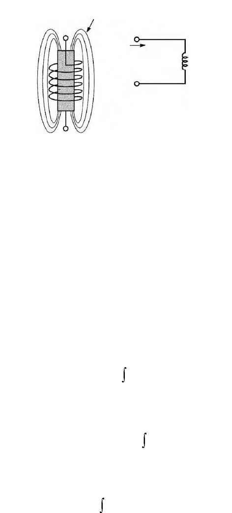
FIGURE 11.40 Iron-core inductor.

Magnetic flux

lines

Circuit

symbol

Iron core

inductor

–

i (t)

(t) = L

t() L

-------

1 H 1 V sec/A=

t()

---

∞–

t = t

()

---

∞–

t()

---

tdI

t ≥ t

9258_C011.fm Page 26 Tuesday, October 2, 2007 4:18 AM

Electrical Engineering 11-27

TABLE 1 1. 4 Analogy between Electrical

and Mechanical Variables

Mechanical System Electrical System

Force, f (N) Current, i (A)

Ve l o c i t y , µ (m/sec) Voltage, v (V)

Damping, B (N sec/m) Conductance, 1/R (S)

Compliance, 1/k (m/N) Inductance, L (H)

Mass, M (kg) Capacitance, C (F)

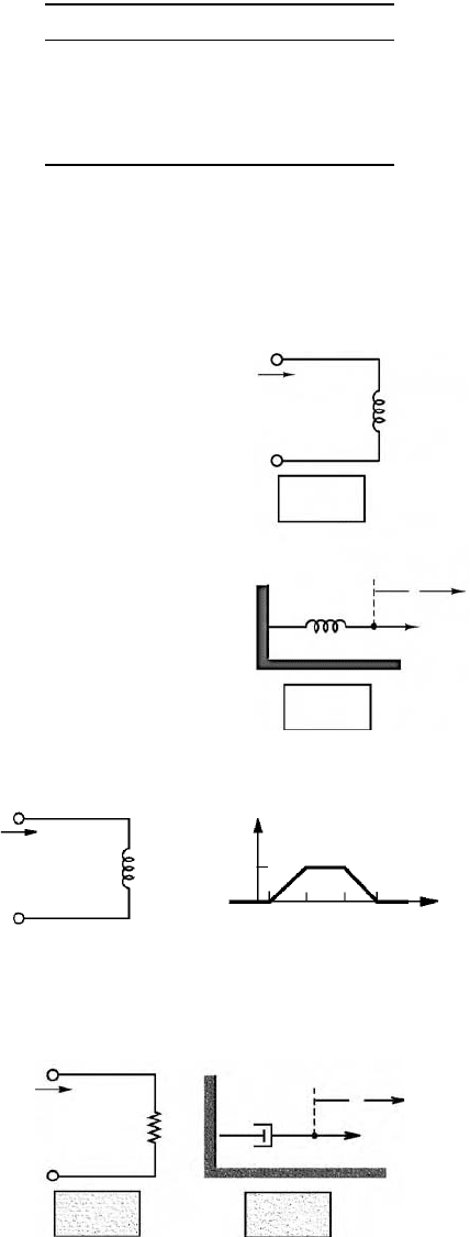
FIGURE 11.41 Defining equation for the ideal induc-

tor and analogy with force–spring system.

FIGURE 11.42 Combining inductors in a circuit.

FIGURE 11.43 Analogy between electrical and mechanical elements.

The defining equation for the

inductance circuit element is

analogous to the equation of

motion of a spring acted upon

by a force.

i (t)

–

i =

∫

u =

f = k

∫

u dt

(t)

i (t)

(A)

01 5 9 13

t (ms)

0.1

–

f = Bu

–

i =

u =

9258_C011.fm Page 27 Tuesday, October 2, 2007 4:18 AM

11-28 Mechatronic Systems, Sensors, and Actuators

11.4.2 Time-Dependent Signal Sources

Figure 11.44 illustrates the convention that will be employed to denote time-dependent signal sources.

One of the most important classes of time-dependent signals is that of periodic signals. These signals

appear frequently in practical applications and are a useful approximation of many physical phenomena.

A periodic signal x(t) is a signal that satisfies the following equation:

(11.41)

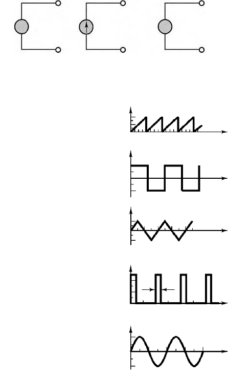
where T is the period of x(t). Figure 11.45 illustrates a number of the periodic waveforms that are typically

encountered in the study of electrical circuits. Waveforms such as the sine, triangle, square, pulse, and

sawtooth waves are provided in the form of voltages (or, less frequently, currents) by commercially

available signal (or waveform) generators. Such instruments allow for selection of the waveform peak

amplitude, and of its period.

As stated in the introduction, sinusoidal waveforms constitute by far the most important class of time-

dependent signals. Figure 11.46 depicts the relevant parameters of a sinusoidal waveform. A generalized

sinusoid is defined as follows:

(11.42)

FIGURE 11.44 Time-dependent signal sources.

FIGURE 11.45 Periodic signal waveforms.

xt() xt nT+()n, 1, 2, 3, …==

xt() A cos

+()=

(t) v (t), i (t )i (t)

––

Generalized time-dependent sources Sinusoidal source

3T 4T

Tim

Sawtooth wave

Square wave

Triangle wave

Pulse train

Tim

2T Tim

Tim

Sine wave

x (t)x (t)

x (t)x (t)x (t)

–A

9258_C011.fm Page 28 Tuesday, October 2, 2007 4:18 AM

Electrical Engineering 11-29

where A is the amplitude,

the radian frequency, and

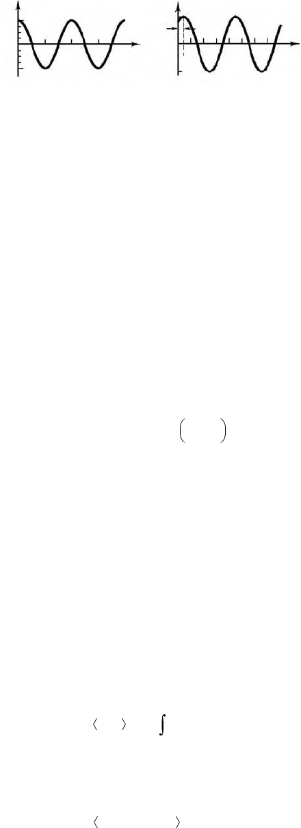
the phase. Figure 11.46 summarizes the

definitions of A,

, and

for the waveforms

where

(11.43)

The phase shift,

, permits the representation of an arbitrary sinusoidal signal. Thus, the choice of the

reference cosine function to represent sinusoidal signals—arbitrary as it may appear at first—does not

restrict the ability to represent all sinusoids. For example, one can represent a sine wave in terms of a

cosine wave simply by introducing a phase shift of

/2 radians:

(11.44)

It is important to note that, although one usually employs the variable ω (in units of radians per

second) to denote sinusoidal frequency, it is common to refer to natural frequency, f, in units of cycles

per second, or hertz (Hz). The relationship between the two is the following:

(11.45)

11.4.2.1 Average and RMS Values

Now that a number of different signal waveforms have been defined, it is appropriate to define suitable

measurements for quantifying the strength of a time-varying electrical signal. The most common types

of measurements are the average (or DC) value of a signal waveform, which corresponds to just measuring

the mean voltage or current over a period of time, and the root-mean-square (rms) value, which takes

into account the fluctuations of the signal about its average value. Formally, the operation of computing

the average value of a signal corresponds to integrating the signal waveform over some (presumably, suitably

chosen) period of time. We define the time-averaged value of a signal x(t) as

(11.46)

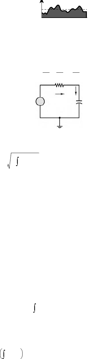
where T is the period of integration. Figure 11.47 illustrates how this process does, in fact, correspond

to computing the average amplitude of x(t) over a period of T seconds.

FIGURE 11.46 Sinusoidal waveforms.

Reference cosine Arbitrary sinusoid

(t)

–A

∆t

–A

t() A cos

t()and x

t() A cos

+()==

f natural frequency

---

cycles/sec, or Hz()==

radian frequency 2

f radians/sec()==

∆T

-------

radians()360

∆T

-------

degrees()==

A sin

t() A cos

---–

xt()

---

xt() td

+()cos 0=

9258_C011.fm Page 29 Tuesday, October 2, 2007 4:18 AM

11-30 Mechatronic Systems, Sensors, and Actuators

A useful measure of the voltage of an AC waveform is the rms value of the signal, x(t), defined as follows:

(11.47)

Note immediately that if x(t) is a voltage, the resulting x

rms

will also have units of volts. If you analyze

Equation 11.47, you can see that, in effect, the rms value consists of the square root of the average (or

mean) of the square of the signal. Thus, the notation rms indicates exactly the operations performed on

x(t) in order to obtain its rms value.

11.4.3 Solution of Circuits Containing Dynamic Elements

The major difference between the analysis of the resistive circuits and circuits containing capacitors and

inductors is now that the equations that result from applying Kirchhoff’s laws are differential equations,

as opposed to the algebraic equations obtained in solving resistive circuits. Consider, for example, the

circuit of Figure 11.48 which consists of the series connection of a voltage source, a resistor, and a

capacitor. Applying KVL around the loop, we may obtain the following equation:

(11.48)

Observing that i

= i

, Equation 11.48 may be combined with the defining equation for the capacitor

(Equation 4.6) to obtain

(11.49)

Equation 11.49 is an integral equation, which may be converted to the more familiar form of a differential

equation by differentiating both sides of the equation, and recalling that

(11.50)

FIGURE 11.47 Averaging a signal waveform.

FIGURE 11.48 Circuit containing energy-storage

element.

(t)

< x (t) >

A circuit containing energy-storage

elements is described by a

differential equation. The

differential equation describing the

series RC circuit shown is

(t )

+ v

–

rms

---

t() td

t() v

t()+=

t() Ri

t()

---

∞–

----

∞–

t()=

9258_C011.fm Page 30 Tuesday, October 2, 2007 4:18 AM

Electrical Engineering 11-31

to obtain the following differential equation:

(11.51)

where the argument (t) has been dropped for ease of notation.

Observe that in Equation 11.51, the independent variable is the series current flowing in the circuit,

and that this is not the only equation that describes the series RC circuit. If, instead of applying KVL,

for example, we had applied KCL at the node connecting the resistor to the capacitor, we would have

obtained the following relationship:

(11.52)

(11.53)

Note the similarity between Equations 11.51 and 11.53. The left-hand side of both equations is identical,

except for the dependent variable, while the right-hand side takes a slightly different form. The solution

of either equation is sufficient, however, to determine all voltages and currents in the circuit.

We can generalize the results above by observing that any circuit containing a single energy-storage

element can be described by a differential equation of the form

(11.54)

where y(t) represents the capacitor voltage in the circuit of Figure 11.48 and where the constants a

and

consist of combinations of circuit element parameters. Equation 11.54 is a first-order ordinary

differential equation with constant coefficients.

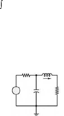
Consider now a circuit that contains two energy-storage elements, such as that shown in Figure 11.49.

Application of KVL results in the following equation:

(11.55)

Equation 11.55 is called an integro-differential equation because it contains both an integral and a

derivative. This equation can be converted into a differential equation by differentiating both sides, to

obtain:

(11.56)

FIGURE 11.49 Second-order circuit.

-------

---

-------

–

---------------

--------

===

--------

-------

dy t()

------------

t()+ Ft()=

Ri t() L

di t()

-----------

---

it()dt

∞–

++ v

t()=

di t()

-----------

it()

-------------

---

it()++

t()

--------------

–

(t )

9258_C011.fm Page 31 Tuesday, October 2, 2007 4:18 AM

11-32 Mechatronic Systems, Sensors, and Actuators

or, equivalently, by observing that the current flowing in the series circuit is related to the capacitor

voltage by i(t) = Cdv

/dt, and that Equation 11.55 can be rewritten as

(11.57)

Note that although different variables appear in the preceding differential equations, both Equations 11.55

and 11.57 can be rearranged to appear in the same general form as follows:

(11.58)

where the general variable y(t) represents either the series current of the circuit of Figure 11.49 or the

capacitor voltage. By analogy with Equation 11.54, we call Equation 11.58 a second-order ordinary

differential equation with constant coefficients. As the number of energy-storage elements in a circuit

increases, one can therefore expect that higher-order differential equations will result.

11.4.5 Phasors and Impedance

In this section, we introduce an efficient notation to make it possible to represent sinusoidal signals as

complex numbers, and to eliminate the need for solving differential equations.

11.4.5.1 Phasors

Let us recall that it is possible to express a generalized sinusoid as the real part of a complex vector

whose argument, or angle, is given by (

t +

) and whose length, or magnitude, is equal to the peak

amplitude of the sinusoid. The complex phasor corresponding to the sinusoidal signal Acos(

t +

)

is therefore defined to be the complex number Ae

(11.59)

1. Any sinusoidal signal may be mathematically represented in one of two ways: a time-domain form

and a frequency-domain (or phasor) form

2. A phasor is a complex number, expressed in polar form, consisting of a magnitude equal to the

peak amplitude of the sinusoidal signal and a phase angle equal to the phase shift of the sinusoidal

signal referenced to a cosine signal.

3. When using phasor notation, it is important to make a note of the specific frequency,

, of the

sinusoidal signal, since this is not explicitly apparent in the phasor expression.

11.4.5.2 Impedance

We now analyze the i–v relationship of the three ideal circuit elements in light of the new phasor notation.

The result will be a new formulation in which resistors, capacitors, and inductors will be described in

the same notation. A direct consequence of this result will be that the circuit theorems of Section 11.3

will be extended to AC circuits. In the context of AC circuits, any one of the three ideal circuit elements

--------

t()

------------------

t()++v

t()=

yt()

--------------

dy t()

------------

yt()++ Ft()=

complex phasor notation for A

+()cos=

vt() A

+()cos=

V j

() Ae

9258_C011.fm Page 32 Tuesday, October 2, 2007 4:18 AM

Electrical Engineering 11-33

defined so far will be described by a parameter called impedance, which may be viewed as a complex

resistance. The impedance concept is equivalent to stating that capacitors and inductors act as frequency-

dependent resistors, that is, as resistors whose resistance is a function of the frequency of the sinusoidal

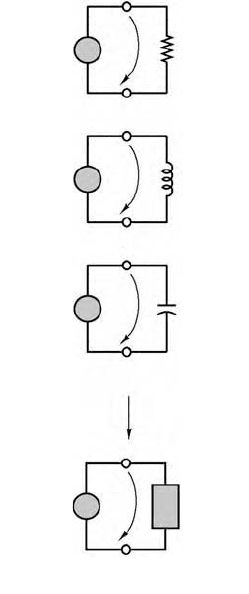
excitation. Figure 11.50 depicts the same circuit represented in conventional form (top) and in phasor-

impedance form (bottom); the latter representation explicitly shows phasor voltages and currents and

treats the circuit element as a generalized “impedance.” It will presently be shown that each of the three

ideal circuit elements may be represented by one such impedance element.

Let the source voltage in the circuit of Figure 11.50 be defined by

(11.60)

without loss of generality. Then the current i(t) is defined by the i–v relationship for each circuit element.

Let us examine the frequency-dependent properties of the resistor, inductor, and capacitor, one at a time.

The impedance of the resistor is defined as the ratio of the phasor voltage across the resistor to the

phasor current flowing through it, and the symbol Z

is used to denote it:

(11.61)

The impedance of the inductor is defined as follows:

(11.62)

FIGURE 11.50 The impedance element.

AC circuits

AC circuits in

phasor / impedance form

Z is the

impedance

of each

circuit

element

∼

–

∼

–

∼

–

∼

–

(t )

i(t )

( j )

I ( j )

t() A

t or V

()cos Ae

()

I j

()

------------------

R==

()

I j

()

------------------

j90°

L===

9258_C011.fm Page 33 Tuesday, October 2, 2007 4:18 AM

11-34 Mechatronic Systems, Sensors, and Actuators

Note that the inductor now appears to behave like a complex frequency-dependent resistor, and that the

magnitude of this complex resistor,

L, is proportional to the signal frequency,

. Thus, an inductor will

“impede” current flow in proportion to the sinusoidal frequency of the source signal. This means that

at low signal frequencies, an inductor acts somewhat like a short circuit, while at high frequencies it tends

to behave more as an open circuit. Another important point is that the magnitude of the impedance of

an inductor is always positive, since both L and

are positive numbers. You should verify that the units

of this magnitude are also ohms.

The impedance of the ideal capacitor, Z

), is therefore defined as follows:

(11.63)

where we have used the fact that 1/j = e

–j90°

= –j. Thus, the impedance of a capacitor is also a frequency-

dependent complex quantity, with the impedance of the capacitor varying as an inverse function of

frequency, and so a capacitor acts like a short circuit at high frequencies, whereas it behaves more like

an open circuit at low frequencies. Another important point is that the impedance of a capacitor is always

negative, since both C and ω are positive numbers. You should verify that the units of impedance for a

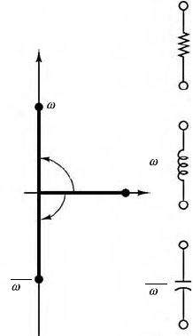
capacitor are ohms. Figure 11.51 depicts Z

(jω) in the complex plane, alongside Z

) and Z

The impedance parameter defined in this section is extremely useful in solving AC circuit analysis

problems, because it will make it possible to take advantage of most of the network theorems developed

for DC circuits by replacing resistances with complex-valued impedances. In its most general form, the

impedance of a circuit element is defined as the sum of a real part and an imaginary part:

(11.64)

where R is called the AC resistance and X is called the reactance. The frequency dependence of R and X

has been indicated explicitly, since it is possible for a circuit to have a frequency-dependent resistance.

The examples illustrate how a complex impedance containing both real and imaginary parts arises in a

circuit.

Example 11.4 Capacitive Displacement Transducer

In Example 11.3, the idea of a capacitive displacement transducer was introduced when we considered

a parallel-plate capacitor composed of a fixed plate and a movable plate. The capacitance of this variable

capacitor was shown to be a nonlinear function of the position of the movable plate, x (see Figure 11.39).

FIGURE 11.51 Impedances of R, L, and C in the com-

plex plane.

90°

–90°

= R

= j L

–

j C

()

I j

()

------------------

--------

j– 90°

j–

--------

----------

== ==

() Rj

()jX j

()+=

9258_C011.fm Page 34 Tuesday, October 2, 2007 4:18 AM

Electrical Engineering 11-35

In this example, we show that under certain conditions the impedance of the capacitor varies as a linear

function of displacement, that is, the movable-plate capacitor can serve as a linear transducer.

Recall the expression derived in Example 11.3:

where C is the capacitance in picofarad, A is the area of the plates in square millimeter, and x is the

(variable) distance in millimeter. If the capacitor is placed in an AC circuit, its impedance will be

determined by the expression

so that

Thus, at a fixed frequency

, the impedance of the capacitor will vary linearly with displacement. This

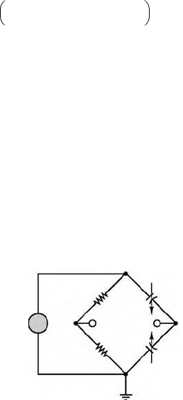
property may be exploited in the bridge circuit of Example 11.3, where a differential pressure transducer

was shown as being made of two movable-plate capacitors, such that if the capacitance of one increased

as a consequence of a pressure differential across the transducer, the capacitance of the other had to decrease

by a corresponding amount (at least for small displacements). The circuit is shown again in Figure 11.52

where two resistors have been connected in the bridge along with the variable capacitors (denoted by

C(x)). The bridge is excited by a sinusoidal source.

Using phasor notation, we can express the output voltage as follows:

If the nominal capacitance of each movable-plate capacitor with the diaphragm in the center position is

given by

where d is the nominal (undisplaced) separation between the diaphragm and the fixed surfaces of the

capacitors (in mm), the capacitors will see a change in capacitance given by

FIGURE 11.52 Bridge circuit for capacitive displace-

ment transducer.

8.854 10

3–

× A

---------------------------------

----------

8.854 j

--------------------------

out

() V

()

x()

----------------------------------

-----------------–

------

dx–

-----------

and C

dx+

------------

(x)

–

)

out

(t)

9258_C011.fm Page 35 Tuesday, October 2, 2007 4:18 AM