Bennett A.F. Inverse Modeling of the Ocean and Atmosphere

Подождите немного. Документ загружается.

2.6 Smoothing norms, covariances and convolutions 57

Think of C

as the covariance of solutions of the model Mu = f , where f has covari-

ance C

. We can now identify the effectively hypothesized covariance:

J [u] = u ◦ C

−1

◦ u + u ◦ B

−1

◦ u +··· (2.6.33)

= u ◦ A

−1

◦ u, (2.6.34)

where



−1

+ B

−1



−1

(2.6.35)

is the harmonic mean of the two covariances C

and B

Chapter 3

Implementation

It is a long road from deriving the formulae for the generalized inverse of a model

and data to seeing results. First experiments (McIntosh and Bennett, 1984) involved

a linear barotropic model separated in time, simple coarsely-resolved numerical ap-

proximations, a handful of pointwise measurements of sea level and a serial computer.

Contemporary models of oceanic and atmospheric circulation involve nonlinear dy-

namics and parameterizations, advanced high-resolution numerical approximations,

vast quantities of data often of a complex nature, and parallel computers. Chapter 3

introduces some general principles for travelling this long road of implementation.

The ﬁrst principle is accelerating the representer algorithm by task decomposition,

that is, by simultaneous computation of representers on parallel processors. The ob-

jective may be either the full representer matrix as required by the direct algorithm,

or a partial matrix for preconditioning the indirect algorithm. The calculation of an

individual representer, or indeed any backward or forward integration, may itself be

accelerated by domain decomposition, but this is a common challenge in modern nu-

merical computation (Chandra et al., 2001; Pacheco, 1996) and will not be addressed

here. Even without considering the coarse grain of task decomposition or the ﬁne grain

of domain decomposition, the direct and indirect representer algorithms for linear in-

verses are highly intricate. Schematics are provided here in the form of “time charts”.

Dynamical errors and input errors may be correlated in space or in time or in both.

Error covariances must be convolved with adjoint variables. This is a massive task if

four dimensions are involved and the numerical resolution is ﬁne. Fast convolutions

are critical to the scientiﬁc purpose of least-squares inversion, which is the testing of

hypotheses about model errors. Posterior error statistics are equally essential, and are

also massively expensive to compute and store in full detail. These statistics need not

3.1 Accelerating the representer calculation 59

be computed with the same precision as the inverse itself, as they are only used for

rough assessment of the likely accuracy of the inverse. Storage-efﬁcient Monte Carlo

algorithms permit computations of selected statistics with adequate reliability, on the

same grid as the forward model if so desired.

Nonlinearity can only be overcome by iteration, but there is no unique way to

iterate. This is a blessing in disguise, as certain choices for functional iterations can

lead to linear, unbounded instability. No functional linearization yields statistical lin-

earization, so signiﬁcance tests and posterior error covariances that assume statistical

linearity must be used with caution. Finally, crude parameterizations of unresolved

natural processes may not be functionally smooth, thereby precluding variational as-

similation. This obstacle should in principle be overcome by ﬁddling with the unnatural

parameterization. Experience with trivial models suggests that we have much to learn.

3.1

Accelerating the representer calculation

3.1.1 So many representers ...

The representer algorithm provides an explicit solution of linear Euler–Lagrange equa-

tions, and hence least-squares generalized inverses of overdetermined linear forward

problems. There is one representer for each excess datum, and two model integrations

are required (one backward, one forward) in order to construct each representer. (Note

that we may regard the initial values and boundary values for the forward problem as

data having exactly the same status as the ﬁnite set of measurements that overdetermine

the forward problem; indeed, we may in principle envisage measurements obtained con-

tinuously along a track, and we shall in Chapter 6 consider specifying boundary values

of too many components of a vector ﬁeld.) It is impractical to compute every repre-

senter if their number is very large. There are rational approaches to reducing their

number, as will be indicated in Chapter 5, but such approximations may not be neces-

sary. It is possible to compute the representer solution for the inverse without reducing

the number of representers, and without signiﬁcant numerical approximation beyond

that already implied by the numerical model. This technical advance has allowed the

inversion of large data sets, with complex models imposed as weak constraints.

3.1.2

Open-loop maneuvering: a time chart

Recall again from §1.3.3 the representer solution for the inverse:

u(x, t) = u

(x, t) +



m=1

(x, t), (3.1.1)

where

(R + C



)

β = h ≡ d − L[u

]. (3.1.2)

60 3. Implementation

Thus our tasks are:

(1) integrate the forward model for u

... one integration;

(2) integrate the backward model for α ... M integrations;

(3) integrate the forward model for r ... M integrations;

for a total of ... I = 2M + 1 integrations.

The backward and forward parts of the Euler–Lagrange equations are coupled by

M numbers

,...,

. The vector coefﬁcient of the impulses in the adjoint equation

(2.4.19), or coupling vector, is actually

−1



(d − L[

u]) = C

−1



{d − L[u

] − R

β} (3.1.3)

= C

−1



{h − R

(R + C



)

−1

... = (R + C



)

−1

β. (3.1.4)

That is, the coupling vector is the vector of representer coefﬁcients. So we need not

store the representer vector ﬁeld r(x, t). We must compute r(x, t), measure it to obtain

the representer matrix R = L[r

], solve (3.1.2) for

β, integrate the adjoint or backward

EL equation (2.4.19) for

λ(x, t) and then integrate the forward equation (1.5.14) for

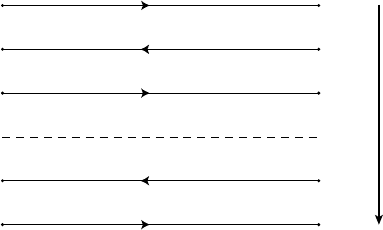
u(x, t). Now the integration count is I = 2M + 3. See Fig. 3.1.1 for a “time chart”

implementing this so-called “open loop” version of the representer algorithm.

t=0 t=T

(1.2.3)

(1.3.9)

(1.3.2)

(1.3.5)

(1.3.12)

(1.2.2) & (1.2.4) u

(1.3.4) & (1.3.6) u

(1.3.1) & (1.3.3) λ

(1.3.8) & (1.3.10) α

,1≤m≤M

(1.3.11) & (1.3.13) r

m,1≤m≤M

(3.1.2) R , β

Figure 3.1.1 Time chart for implementing the representer

algorithm with direct calculation of the representer

coefﬁcient

β, that is, by explicit or direct construction of the

representer matrix R. The heavy vertical arrow on the right

indicates the order of execution, which starts at the top. Note

that (3.1.1) need not be summed explicitly; once

β is

known, (3.1.4) resolves the coupling in (1.3.1)–(1.3.6). So in

this “open loop” version, λ and hence

u may be calculated

with one backward integration and one forward integration.

The representers r

,1≤ m ≤ M, need not be stored. If the

inverse weights W

−1

, W

−1

and w

−1

are nondiagonal, then

(1.3.11)–(1.3.13) and (1.3.4)–(1.3.6) require convolutions as

in (1.5.14)–(1.5.16). See also (4.2.1)–(4.2.6) for a statement

of the Euler–Lagrange equations for nondiagonal weighting.

3.1 Accelerating the representer calculation 61

Table 3.1.1 Processor work sheet.



··· 

L[r

] L[r

]

(all processors get the other M−1 columns of R)

(all processors solve for

β = (R + C



)

−1

(d − L[u

]))

λλ λ

I = 5 I = 5 I = 5

3.1.3 Task decomposition in parallel

The above task is ideally suited to parallel processing (Bennett and Baugh, 1992). Sup-

pose we have M processors 

,...,

. The work sheet is as follows (see Table 3.1.1).

The m

processor 

calculates the ﬁelds u

,α

and r

, takes all M measurements

,...,L

of r

to obtain the m

column of R, broadcasts this column to all of

the other M −1 processors, receives the other M −1 columns in return, assembles R,

solves for the vector

β, then solves the Euler–Lagrange equations by calculating the

ﬁeld λ and the ﬁeld

So I is reduced from 2M + 3 to 5 with an M-processor system. There is minimal

exchange of data: each processor broadcasts one column of the representer matrix, and

receives M −1 columns in return. Each processor 

must have sufﬁcient memory and

speed for the computation and storage of u(x, t), for 0 ≤ x ≤ L and 0 ≤ t ≤ T . Note

that the calculations of u

, λ and

u are M-fold redundant. This permits the programmer

to release M −1 processors during these steps; more importantly it permits a reduction

of the number of broadcast messages by a factor of M −1.

3.1.4

Indirect representer algorithm; an iterative time chart

Generalized inversion reduces exactly to solving the ﬁnite-dimensional system

(R + C



)

β = (d − L[u

]), (3.1.5)

or simply

β = h. (3.1.6)

A direct solution requires that P and hence R be explicitly known. However, the solution

may be obtained iteratively, provided Pψ can be evaluated for any vector ψ. Then a

standard iterative solver can convert a ﬁrst-guess

into a solution

β = P

−1

62 3. Implementation

Let us now examine how we could compute Pψ, given any vector ψ.Wehave

Pψ = Rψ + C



ψ. (3.1.7)

The data error covariance matrix C



is explicitly known, so the nontrivial problem is

the evaluation of Rψ. The following procedure (Egbert et al., 1994; Amodei, 1995;

Courtier, 1997) does that without calculating the representers. First, solve the backward

model, with coupling vector ψ:

−

∂φ

∂t

− c

∂φ

∂x

= ψ

LL[δδ], (3.1.8)

subject to

φ = 0 (3.1.9)

at t = T , and

φ = 0 (3.1.10)

at x = L. Second, solve the forward model, with adjoint ﬁeld φ(x , t):

∂θ

∂t

+ c

∂θ

∂x

= C

• φ, (3.1.11)

subject to

θ = C

◦ φ (3.1.12)

at t = 0, and

θ = cC

∗ φ (3.1.13)

at x = 0. Comparison of (3.1.8)–(3.1.13), with the equations (2.4.14), (2.4.13) for α

and r respectively, shows that

φ(x, t) = ψ

α(x, t),θ(x, t) = ψ

r(x, t) = r(x, t)

ψ. (3.1.14)

Hence

L[θ] = L[r

]ψ = Rψ, (3.1.15)

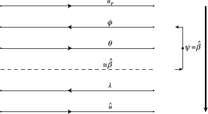
which is just what is needed, at a cost of two integrations; see Fig. 3.1.2.

3.1.5

Preconditioners

If P is the unit matrix, then iterative solution of (3.1.6) should converge to h in one

step. Hence iteration on (3.1.6) should in general be accelerated by premultiplying both

sides of (3.1.6) with the inverse of a symmetric, positive-deﬁnite approximation to P.

That is, solve

−1

β = P

−1

h, (3.1.16)

3.1 Accelerating the representer calculation 63

t=0 t=T

(1.2.3)

(3.1.9)

(1.3.2)

(1.3.5)

(3.1.12)

(1.2.2) & (1.2.4)

(1.3.4) & (1.3.6)

(1.3.1) & (1.3.3)

(3.1.8) & (3.1.10)

(3.1.11) & (3.1.13)

(3.1.15) & (3.1.7)

Figure 3.1.2 Time chart for implementing the indirect

representer algorithm. The representer coefﬁcients

β are

approximated by iterative solution of (3.1.2). Given a previous

approximation ψ for

β, the “inner iteration” calculates

Pψ = Rψ + C



ψ with one backward integration and one

forward integration (the representer matrix R is not explicitly

constructed). This information is then used to ﬁnd a better

approximation ψ



for

β. Once

β has been approximated with

sufﬁcient accuracy, λ and hence

u are calculated as in the direct

“open loop” algorithm. That is, the sum (3.1.1) is evaluated

implicitly by one backward integration and one forward

integration.

where P

∼

P. Then (3.1.16) may be solved iteratively since, if we can evaluate Pψ

for any ψ, then we can also evaluate P

−1

Pψ. There are various choices for the pre-

conditioner P

(i) (Bennett et al., 1996) We could calculate all the representers quickly and

cheaply on a coarse grid. Note that we would still be in effect solving (3.1.6) for

the coefﬁcients of the representers on the ﬁne grid, so there would be no loss of

resolution in

u(x, t). However, the grid vertices may not coincide very closely

with observing sites; the measurement functionals must involve interpolation

formulae and these degrade appreciably as the grid gets coarser. That is, P

may be a poor approximation to P and so convergence may not be greatly

accelerated.

(ii) (Egbert and Bennett, 1996; Egbert, 1997) We could calculate some of the

representers on the ﬁne grid. Let R

be the M × K matrix consisting of the ﬁrst

K columns of R. That is, R = (R

, R

), where the non-calculated matrix R

is of dimension M × (M − K ). Now R

may be partitioned into an upper

K × K block denoted by R

, and a lower (M − K ) × K block R

, etc.

That is,

R =





= (R

, R

). (3.1.17)

64 3. Implementation

The representer matrix is symmetric, therefore R

is actually known at this

point: R

= R

. An estimate for R

is R

−1

, thus



−1



. (3.1.18)

Then P

= R

+ C



. Note that the ranks of R

and P

are K and M

respectively. The effectiveness of this preconditioner depends upon a judicious

choice for the K calculated representers, and upon the independence of the

measurement errors.

(iii) Recall from (2.2.9) and (2.4.18) that the representer matrix is a covariance:

R = LC

(3.1.19)

= E{(L[u] − L[u

])(L[u] − L[u

])

}. (3.1.20)

Thus we may estimate R by Monte Carlo methods. That is, we make

pseudo-random samples of L[u − u

] and then evaluate sample covariances.

The issue is: how many samples sufﬁce?

Further details on implementation, including a ﬂowchart, may be found in Chapter 5.

The issue of sample size will be illustrated in §5.5.

3.1.6

Fast convolutions

We have seen the need to assume “nondiagonal” covariances for dynamical errors;

that is,

(x, t, x



, t



) = δ(x − x



)δ(t − t



). (3.1.21)

The covariance appears in the “forward” equation for the inverse estimate, for example

(1.5.14):

∂

∂t

(x, t) +c

∂

∂x

(x, t) = F(x, t) + (C

• λ)(x, t), (3.1.22)

where

• λ)(x, t) =



dy C

(x, t, y, s)λ(y, s). (3.1.23)

Direct evaluation of this integral for each (x, t) would be prohibitively expensive in only

one space dimension and time, and even more so in several space dimensions and time.

Thus, a crucial requirement for smooth and hence physically acceptable inversions is

an efﬁcient algorithm for the evaluation of integrals such as (3.1.23). We shall refer to

these loosely as “convolutions”.

The following shortcut is very efﬁcient (Derber and Rosati, 1989; Egbert et al.,

1994). Assume that the covariance is purely spatial, and is “bell-shaped”:

C(x, x



) = C

exp(−|x − x



), (3.1.24)

3.1 Accelerating the representer calculation 65

where C

is a constant. Assume that we wish to evaluate

b(x) =

∞



−∞

∞



−∞

C(x, x



)a(x



) dx



. (3.1.25)

Solve the following pseudo-heat equation for θ = θ(x, s):

∂θ

∂s

=∇

θ, (3.1.26)

by time-stepping, subject to

θ(x, 0) = a(x). (3.1.27)

In two space dimensions, the solution is

θ(x, s) = (4π s)

−1

∞



−∞

∞



−∞

exp(−|x − x



/(4s))a(x



) dx



. (3.1.28)

So let

s = L

/4, (3.1.29)

then

b(x) = π L

θ(x, L

/4). (3.1.30)

Exercise 3.1.1

Compare the operation counts for numerical integration of (3.1.26), and numerical

evaluation of (3.1.25), for one, two and three space dimensions. 

Exercise 3.1.2

How might you proceed when the spatial domain is ﬁnite? 

If the covariance is inhomogeneous, for example

C(x, x



) = V (x)

V (x



)

exp(−|x − x



), (3.1.31)

where V (x) = C(x, x) is the variance, then proceed as above except that the initial

condition becomes

θ(x, 0) = V (x)

a(x), (3.1.32)

and the required result is

b(x) = V (x)

π L

θ(x, L

/4). (3.1.33)

Now consider temporal convolution, involving the simple form

C(t, t



) = exp(−|t − t



|/τ ).

66 3. Implementation

That is, we wish to evaluate

b(t) =



C(t, t



)a(t



) dt



. (3.1.34)

This is the solution of

− τ

−2

b =−2τ

−1

a (3.1.35)

for 0 ≤ t ≤ T , subject to

− τ

−1

b = 0 (3.1.36)

at t = 0, and

+ τ

−1

b = 0 (3.1.37)

at t = T . The two point boundary-value problem (3.1.35)–(3.1.37) is easily solved as

two initial-value problems. First, solve

+ τ

−1

h =−2τ

−1

a (3.1.38)

for 0 ≤ t ≤ T , subject to

h = 0 (3.1.39)

at t = 0. Then solve

− τ

−1

b = h (3.1.40)

for 0 ≤ t ≤ T , subject to

b =−(τ/2)h (3.1.41)

at t = T .

Exercise 3.1.3

Show that the order of the two integrations in Exercise 3.1.2 may be reversed, with a

modiﬁcation to the terminal conditions. 

3.2

Posterior errors

3.2.1 Strategy

How good is the generalized inverse

u?Ifu is the true circulation, and if we adopt the

statistical interpretation of the inverse, then the error u −

u has zero mean. There is a

closed expression for the covariance of this error, or posterior error covariance. The