Bennett A.F. Inverse Modeling of the Ocean and Atmosphere
Подождите немного. Документ загружается.


1.5 Regularity of the inverse estimate 27
T
L0
t
x
(x
m
, t
m
)
t
m
-c
-1
x
m
Figure 1.5.1 Support of
α
m
(x , t ). The arrows (the
delta functions) are normal
to the page.
T
L
0
t
x
(x
M
, t
M
)
(x
m
, t
m
)
(x
1
, t
1
)
(x
3
, t
3
)
(x
2
, t
2
)
(x
4
, t
4
)
Figure 1.5.2 Support of
singularities in
ˆ
u(x, t).
subject to the initial and boundary conditions
ˆ
u = I +
ˆ
ı = I + W
−1
i
λ,
ˆ
u = B +
ˆ
b = B + cW
−1
b
λ. (1.5.6)
So our estimates of
ˆ
f ,
ˆ
ı and
ˆ
b are singular. There is neither dispersion nor diffusion
in our “toy” ocean dynamics, so
ˆ
u is also singular: see Fig. 1.5.2. This is hardly a
satisfactory combination of dynamics and data!
Exercise 1.5.1
Express r
m
and
ˆ
u using the Green’s function γ .
1.5.3
Nondiagonal weighting: kernel inverses of weights
We want the data to influence the circulation at remote places and times, so we should
give weight to products of residuals at remote places and times. We therefore generalize

28 1. Variational assimilation
the penalty functional (1.2.9) to
J [u] =
T
0
dt
T
0
ds
L
0
dx
L
0
dy f (x, t)W
f
(x, t, y, s) f (y, s)
+
L
0
dx
L
0
dy i(x)W
i
(x, y)i(y) +
T
0
dt
T
0
ds b(t)W
b
(t, s)b(s)
+
M
l=1
M
m=1
l
w
lm
m
. (1.5.7)
Thus our previous, trivial choices were
W
f
(x, t, y, s) = W
f
· δ(x − y)δ(t − s), etc. (1.5.8)
The notations
•≡
T
0
dt
L
0
dx, ◦≡
L
0
dx, ∗≡
T
0
dt
allow us to write J more compactly as
J [u] = f • W
f
• f + i ◦ W
i
◦ i + b ∗ W
b
∗ b +
T
w. (1.5.9)
Exercise 1.5.2
Define the weighted residual or adjoint variable λ(x, t )by
λ ≡ W
f
•
∂
ˆ
u
∂t
+ c
∂
ˆ
u
∂x
− F
. (1.5.10)
Then show that the Euler–Lagrange equations for minima of (1.5.9) are just as
before.
Exercise 1.5.3
Define C
f
, the inverse of W
f
,by
C
f
• W
f
≡
T
0
dr
L
0
dz C
f
(x, t, z, r)W
f
(z, r, y, s) (1.5.11)
= δ(x − y)δ(t − s) . (1.5.12)
Define C
i
and C
b
analogously, and define C
by
wC
= I . (1.5.13)

1.5 Regularity of the inverse estimate 29
Each entity in (1.5.13) is an M × M matrix. Now, write out the representer solution
of the Euler–Lagrange equations. Verify that the solution only requires C
f
, C
i
, C
b
and
C
; that is, it does not require their inverses, the weights W
f
, W
i
, W
b
and w.
1.5.4
The inverse weights smooth the residuals
The inverse estimate
ˆ
u obeys
∂
ˆ
u
∂t
(x, t) +c
∂
ˆ
u
∂x
(x, t) = F (x, t) + (C
f
• λ)(x, t)
= F(x, t) +
T
0
ds
L
0
dy C
f
(x, t, y, s)λ(y, s), (1.5.14)
subject to
ˆ
u(x, 0) = I (x) + (C
i
◦ λ)(x, 0), (1.5.15)
and
ˆ
u(0, t ) = B(t) +c(C
b
∗ λ)(0, t) . (1.5.16)
The supposition is that C
f
, C
i
and C
b
smooth the singular behavior of λ, yielding
regular estimates for
ˆ
f ≡ C
f
• λ,
ˆ
ı ≡ C
i
◦ λ and
ˆ
b = cC
b
∗ λ, leading in turn to a
regular estimate
ˆ
u for the ocean circulation.
In summary, we should avoid “diagonal” weighting.
Note 1. The adjoint variables α and λ remain singular, but r and u should become
regular.
Note 2. Evaluation of the convolutions in (1.5.14), (1.5.15) and (1.5.16) at each
position and time is potentially very expensive: consider three space
dimensions and time.
Note 3. Functional analysis sheds much light on smoothness: see §2.6.
Exercise 1.5.4
Consider slow, viscous flow as discussed in Exercises 1.1.3 and 1.2.2. Construct both
the adjoint representers α and the representers r, using the Green’s function φ given in
(1.1.26). How smooth are α and r? Is nondiagonal weighting of either the dynamical
penalty or the initial penalty necessary?
Exercise 1.5.5
Generalize the definition of the rk given in (1.3.30) et seq. Prove that

30 1. Variational assimilation
(i) r
m
(x, t) = (x, t, x
m
, t
m
), (1.5.17)
for 1 ≤ m ≤ M;
(ii) = γ • C
f
• γ + γ ◦ C
i
◦ γ + c
2
γ ∗ C
b
∗ γ. (1.5.18)
Note:
The adjoint equations (1.3.1)–(1.3.3) and forward equations (1.5.14)–(1.5.16),
which constitute the most general form of the Euler–Lagrange equations devel-
oped in §1.2 and §1.5, are restated for convenience in §4.2 as (4.2.1)–(4.2.6).
Chapter 2
Interpretation
The calculus of variations uses Green’s functions and representers to express the best
fit to a linear model and data. Mathematical construction of the representers is devious,
and the meaning of the representer solution to the “control problem” of Chapter 1 is not
obvious. There is a geometrical interpretation, in terms of observable and unobservable
degrees of freedom. Unobservability defines an orthogonality, and the representers span
a finite-dimensional subspace of the space of all model solutions or “circulations”.
The representers are in fact the observable degrees of freedom.
A statistical interpretation is also available: if the unknown errors in the model
are regarded as random fields having prescribed means and covariances, then the
representers are related, via the measurement processes, to the covariances of the
circulations. Thus the representer solution to the variational problem is also the optimal
linear interpolation, in time and space, of data from multivariate, inhomogeneous and
nonstationary random fields. The minimal value of the penalty functional that defines
the generalized inverse or control problem is a random number. It is the χ
2
variable, if
the prescribed error means or covariances are correct, and has one degree of freedom
per datum. Measurements need not be pointwise values of the circulation; representers
along with their geometrical and statistical interpretations may be constructed for all
bounded linear measurement functionals.
Analysis of the conditioning of the determination of the representer amplitudes
reveals those degrees of freedom which are the most stable with respect to the observa-
tions. This characterization also indicates the efficiency of the observing system – the
fewer unstable degrees of freedom, the better.
Interpreting the variational formulation is completed by demonstrating the relation-
ship between weights, covariances and roughness penalties.
31

32 2. Interpretation
2.1 Geometrical interpretation
2.1.1 Alternatives to the calculus of variations
After formulating the penalty functional that defines the best fit to our model and our
data, we found a local extremum using the theory of the calculus of the first variation.
Specifically, we derived the Euler–Lagrange equations, and explicitly expressed their
solution with representers. These functions were defined as special and directly cal-
culable solutions of Euler–Lagrange-like equations. We shall now construct the same
extremum for the penalty functional using Hilbert Space theory (Yoshida, 1980). This
geometrical construction reveals the efficiency of minimization algorithms based on
the Euler–Lagrange equations.
Exercise 2.1.1
How do we know that we shall find the same extremum?
2.1.2
Inner products
We begin by defining an inner product for two “ocean circulations” u = u(x, t) and
v = v(x, t ):
u,v≡
T
0
dt
T
0
ds
L
0
dx
L
0
dy
∂
∂t
+ c
∂
∂x
u(x, t)
×W
f
(x, t, y, s)
∂
∂s
+ c
∂
∂y
v(y, s)
+
L
0
dx
L
0
dy u(x, 0)W
i
(x, y)v(y, 0)
+
T
0
dt
T
0
ds u(0, t)W
b
(t, s)v(0, s)
= f
u
• W
f
• f
v
+ u ◦ W
i
◦ v + u ∗ W
b
∗ v, (2.1.1)
where f
u
is the residual for u (Bennett, 1992).
Exercise 2.1.2
Verify that , is an inner product, that is:
(i) u,v=v, u (assume the W are symmetric),
(ii) cu + dw, v=cu,v+dw, v for all real numbers c and d,
(iii) u, u≥0,
(iv) u, u=0 ⇔ u ≡ 0 (nontrivial).
2.1 Geometrical interpretation 33
In terms of the inner product, our penalty functional is
J [u] =u − u
F
, u − u
F
+(d − u)
T
w(d − u). (2.1.2)
2.1.3
Linear functionals and their
representers; unobservables
Consider the linear mapping
u → u(ξ,τ), (2.1.3)
where the lhs is a field, while the rhs is a particular value of the field. This mapping is
a linear functional: it linearly maps a function to a single number.
Theorem 2.1.1
If the vector space of admissible fields u, with the inner product , , is complete (that
is, if it is a Hilbert Space), then there is a function ρ(x, t,ξ,τ) such that
ρ,u=u(ξ,τ). (2.1.4)
So ρ “represents” the measurement process. This is the Riesz representation
theorem. Given ρ, we may express J entirely in terms of inner products (Wahba and
Wendelberger, 1980):
J [u] =u − u
F
, u − u
F
+(d −ρ, u)
T
w(d −ρ, u), (2.1.5)
where ρ
m
= ρ(x, t, x
m
, t
m
), 1 ≤ m ≤ M.
Now, any field u = u(x, t) may be expressed as
u(x, t) = u
F
(x, t) +
M
m=1
ν
m
ρ(x, t, x
m
, t
m
) + g(x, t), (2.1.6)
where u
F
is again the solution of (1.2.2)–(1.2.4), and where the ν
m
are any coefficients,
since we may always choose
g ≡ u − u
F
− ν
T
ρ. (2.1.7)
Let us now impose the condition that g is “unobservable”:
ρ
m
, g=g(x
m
, t
m
) = 0 (2.1.8)
for 1 ≤ m ≤ M. That is, g is orthogonal to each ρ
m
. For a given u and a given u
F
,we
may use (2.1.8) to derive M equations for the ν
m
; then g is uniquely defined by (2.1.7).
34 2. Interpretation
2.1.4 Geometric minimization with representers
But we’re not given u; we’re only given u
F
. Thus ν and g are arbitrary. We wish to
find the u that minimizes J [u]. Let us evaluate J using (2.1.5) and (2.1.6):
J [u] =ν
T
ρ + g, ν
T
ρ + g
+(d −ρ, u
F
+ ρ
T
ν + g)
T
w(d −ρ, u
F
+ ρ
T
ν + g)
= ν
T
ρ, ρ
T
ν + ν
T
ρ, g+g, ρ
T
ν +g, g
+(d −ρ, u
F
−ρ, ρ
T
ν −ρ, g)
T
w(d −ρ, u
F
−ρ, ρ
T
ν −ρ, g).
(2.1.9)
Next impose the M orthogonality conditions (2.1.8), and use the representing property
of ρ to obtain
J [u] = J [ν, g] = ν
T
ρ, ρ
T
ν +g, g
+(d − u
F
−ρ, ρ
T
ν)
T
w(d − u
F
−ρ, ρ
T
ν). (2.1.10)
The penalty functional J is now expressed explicitly in terms of ν and g. Note that g
only appears once on the rhs of (2.1.10). Clearly J is least with respect to the choice
of g if g, g=0, that is
g =
ˆ
g ≡ 0. (2.1.11)
We discard the field g orthogonal to all the representers. It remains to select the ν
m
,
1 ≤ m ≤ M. But first note that
σ
lm
≡ρ, ρ
T
lm
=ρ
l
,ρ
m
=ρ
m
,ρ
l
= ρ
m
(x
l
, t
l
) = ρ
l
(x
m
, t
m
)
= σ
ml
, (2.1.12)
so σ = σ
T
and J , which now only depends upon ν, may be expressed as
J [u] = J [ν] = ν
T
σν + (h − σν)
T
w(h − σν), (2.1.13)
where h ≡ d − u
F
. Completing the square,
J [ν] = (ν − ˆν)
T
S(ν − ˆν) + h
T
wh − ˆν
T
S ˆν, (2.1.14)
where S = σ + σwσ and S ˆν = σwh, both of which are given. We finally minimize J
by choosing ν = ˆν, and then
ˆ
J ≡ J [ˆν] = h
T
wh − ˆν
T
S ˆν. Provided σ is nonsingular,
we may untangle these results to find
(σ + w
−1
)ˆν = h, (2.1.15)
which looks familiar.
Recall that our minimizer is
ˆ
u = u
F
+ ˆν
T
ρ +
ˆ
g, (2.1.16)
where
ˆ
g satisfies (2.1.11), and ˆν satisfies (2.1.15).

2.1 Geometrical interpretation 35
2.1.5 Equivalence of variational and geometric
minimization: the data space
Surely the representers ρ defined by the representing property (2.1.4) are the same as
the representer functions r that satisfy the Euler–Lagrange-like system (1.3.8)–(1.3.13),
in which case
σ = R, ˆν =
ˆ
β ? (2.1.17)
Exercise 2.1.3
Show that
ρ
m
(x, t) = r
m
(x, t) (2.1.18)
for 0 ≤ x ≤ L,0≤ t ≤ T , and 1 ≤ m ≤ M.
Hint
Consider (2.1.4):
u(x
m
, t
m
) ≡ρ
m
, u
≡
T
0
dt
T
0
ds
L
0
dx
L
0
dy
∂
∂t
+ c
∂
∂x
ρ
m
(x, t)
×W
f
(x, t, y, s)
∂
∂s
+ c
∂
∂y
u(y, s)
+
L
0
dx
L
0
dy ρ
m
(x, 0)W
i
(x, y)u(y, 0)
+
T
0
dt
T
0
ds ρ
m
(0, t)W
b
(t, s)u(0, s). (2.1.19)
Integrate the first integral by parts, and then compare (2.1.19) to
u(x
m
, t
m
) =
T
0
dt
L
0
dx u(x, t)δ(x − x
m
)δ(t − t
m
). (2.1.20)
Since the partially-integrated (2.1.19) must agree with (2.1.20) for all fields u(x, t)
having initial values u(x, 0) and boundary values u(0, t), we may equate their respective
coefficients, arriving at (1.3.8)–(1.3.13). We have proved that for any field u,
r, u=u. (2.1.21)
36 2. Interpretation
Note 1. We have established that
ˆ
u(x, t) − u
F
(x, t) =
ˆ
β
T
r(x, t). (2.1.22)
That is, the difference between the inverse estimate
ˆ
u and the prior estimate u
F
is a linear combination of the M representers r
1
,...,r
M
. The difference lies in
the observable space, that is, we reject any additional difference g that is
unobservable: r, g=0. We began with a search for the optimal or best-fit
field
ˆ
u(x, t), where 0 ≤ x ≤ L and 0 ≤ t ≤ T . This would be a search amongst
an infinite number of degrees of freedom (the “state space”). We have exactly
reduced the task to a search for the M optimal representer coefficients
ˆ
β
1
,...,
ˆ
β
M
: see Fig. 2.1.1. These are the observable degrees of freedom (the
“data space”).
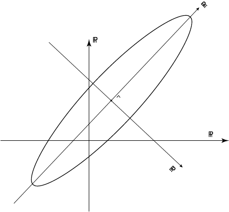
u
Data
State
State
N
u
ll
Figure 2.1.1 The plane represents the state space. It has an
axis u(x, t) for each (x, t) in the intervals 0 ≤ x ≤ L,
0 ≤ t ≤ T . In principle this is an infinite dimensional space.
In practice, when we replace continuous intervals and partial
differential equations with grids and partial difference
equations, the state space usually has a very large but finite
dimension. The contour is defined by a constant value for the
penalty functional J [u], and has principal axes
R
Data
(for β
T
r(x , t )) and R
Null
(for g(x, t)). Note that the
representers r
1
(x , t ),...,r
M
(x , t ) are known, and span the
data space, so only the unknown β
1
,...,β
M
vary in the data
space. The unobservable field g(x , t) is unknown and variable
for 0 ≤ x ≤ L,0≤ t ≤ T . Realizing that
ˆ
g is zero greatly
reduces the size of the search for
ˆ
u, as we need only search in
the data space.