Bennett A.F. Inverse Modeling of the Ocean and Atmosphere
Подождите немного. Документ загружается.


A.1 Forward model 197
A.1.5 Model forcings
The model forcings are
F
u
=−C
d
ρ
a
u
a
2
/(H ρ
w
),
and
F
v
= 0.
A.1.6
Model parameters
The following parameters are suggested:
zonal period, X = 2000 km
meridional width, Y = 1000 km
mean depth, H = 5000 m
time interval, T = 1.8 ×10
4
s
gravitational acceleration, g = 9.806 m s
−2
Coriolis parameter, f = 1.0 × 10
−4
s
−1
damping coefficient, r
u
= (1.8 × 10
4
s)
−1
damping coefficient, r
v
= (1.8 × 10
4
s)
−1
damping coefficient, r
q
= (1.8 × 10
4
s)
−1
drag coefficient, C
d
= 1.6 × 10
−3
air density, ρ
a
= 1.275 kg m
−3
water density, ρ
w
= 1.0 × 10
3
kg m
−3
zonal wind, u
a
= 5ms
−1
.
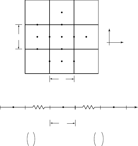
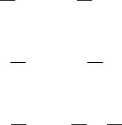
A.1.7 Numerical model
The differential equations are discretized on the Arakawa C-grid (see Fig. A.1.2) with
a forward–backward scheme for time-stepping (Mesinger & Arakawa, 1976) given as
follows:
q
k+1
i, j
− q
k
i, j
t
+ H
u
k
i+1, j
− u
k
i, j
x
+
v
k
i, j +1
− v
k
i, j
y
+r
q
q
k
i, j
= 0,
u
k+1
i, j
− u
k
i, j
t
− f
v
k
i, j +1
+ v
k
i, j
+ v
k
i−1, j +1
+ v
k
i−1, j
4
+ g
q
k+1
i, j
− q
k+1
i−1, j
x
+r
u
u
k
i, j
= F
u
k
i, j
,
v
k+1
i, j
− v
k
i, j
t
+ f
u
k
i+1, j
+ u
k
i, j
+ u
k
i+1, j −1
+ u
k
i, j −1
4
+ g
q
k+1
i, j
− q
k+1
i, j −1
y
+r
v
v
k
i, j
= F
v
k
i, j
,
198 Appendix A Computing exercises
U
0
U
1
U
k-1
U
NK-1
U
NK
U
k
q
i,j+1
q
i,j-1
u
i,j-1
u
i+1,j-1
q
i,j
u
i,j
v
i,j
v
i,j+1
v
i-1,j+1
u
i+1,j
q
i-1,j
q
i+1,j
v
i-1,j
∆y
∆x
∆t
j
i
Spatial:
Temporal:
λ
1
λ
u
λ
v
λ
q
λ
k
λ
NK
U = v
u
q
λ =
k
Figure A.1.2 Arakawa C-grid for space differences; staggering of
forward and adjoint variables for time differences.
where
q
k
i, j
: i = 1, NI; j = 1, NJ − 1; k = 0, NK − 1,
u
k
i, j
: i = 1, NI; j = 1, NJ − 1; k = 0, NK − 1,
and
v
k
i, j
: i = 1, NI ; j = 2, NJ − 1; k = 0, NK − 1.
Rigid boundary conditions
v
k
i,1
= 0,
and
v
k
i,NJ
= 0.
Periodic boundary conditions
u
k
0, j
= u
k
NI, j
,
u
k
NI+1, j
= u
k
1, j
,
v
k
0, j
= v
k
NI, j
,
v
k
NI+1, j
= v
k
1, j
,
q
k
0, j
= q
k
NI, j
,
A.2 Variational data assimilation 199
and
q
k
NI+1, j
= q
k
1, j
.
A.1.8
Numerical model parameters
The following parameters are suggested:
number of grid points in x-direction, NI = 20
number of grid points in y-direction, NJ = 11
number of time steps, NK = 100
grid spacing (x-direction), x = 100 km
grid spacing (y-direction), y = 100 km
time step, t = 180 s.
A.1.9 Numerical code and output
Source code: fwd.f
To compile the source code: f77-O3 fwd.f -o fwd
Output file: ufwd.dat, vfwd.dat and qfwd.dat
A.1.10 To generate a plot
(i) Postprocessing
Source code: postprocess.f
To compile the source code: f77 postprocess.f -o postprocess
Input file: ufwd.dat, vfwd.dat and qfwd.dat
Output file: u.dat, v.dat, q.dat, uy.dat, vy.dat, qy.dat
(ii) Line plot
gnuplot line.gnu (input file: qy.dat; output file: qy.ps)
(iii) Contour plot
gnuplot contour.gnu (input file: q.dat; output file: q.ps)
A.2
Variational data assimilation
A.2.1 Preamble
The exercise is to reformulate the forward model of Exercise A.1 as an inverse model,
to define a penalty functional, to derive the associated system of Euler–Lagrange (EL)
equations and to express its solution using representers.

200 Appendix A Computing exercises
A.2.2 Penalty functional
Formulate the penalty functional J for the following problem (see §1.2, Inverse
models):
Equations of motion
∂u
∂t
− f v + g
∂q
∂x
+r
u
u = F
u
+ f
u
,
∂v
∂t
+ fu+ g
∂q
∂y
+r
v
v = F
v
+ f
v
,
∂q
∂t
+ H
∂u
∂x
+
∂v
∂y
+r
q
q = f
q
.
Initial conditions
u(x, y, 0) = I
u
(x, y) + i
u
(x, y),
v(x, y, 0) = I
v
(x, y) + i
v
(x, y),
q(x, y, 0) = I
q
(x, y) + i
q
(x, y).
Rigid boundary conditions
v(x, 0, t ) = b
0
(x, t),
v(x, Y, t) = b
Y
(x, t).
Periodic boundary conditions
u(x ± X, y, t) = u(x, y, t),
v(x ± X, y, t) = v(x, y, t),
q(x ± X, y, t) = q(x, y, t).
Data
d
m
= q(x
m
, y
m
, t
m
) +
m
, 1 ≤ m ≤ M.
A.2.3
Euler–Lagrange equations
Derive EL equations for the extremum of the penalty functional J .
A.2.4
Representer solution
Solve the EL equations using representers (see §1.3: Solving the Euler–Lagrange equa-
tions using representers).
A.2 Variational data assimilation 201
A.2.5 Solutions for A.2.2–A.2.4
Penalty functional, in terms of residuals:
J = J [u,v,q]
= W
u
f
T
0
dt
X
0
dx
Y
0
dy( f
u
(x, y, t))
2
+ W
v
f
T
0
dt
X
0
dx
Y
0
dy( f
v
(x, y, t))
2
+W
q
f
T
0
dt
X
0
dx
Y
0
dy( f
q
(x, y, t))
2
+ W
u
i
X
0
dx
Y
0
dy(i
u
(x, y))
2
+W
v
i
X
0
dx
Y
0
dy(i
v
(x, y))
2
+ W
q
i
X
0
dx
Y
0
dy(i
q
(x, y))
2
+W
v
b
T
0
dt
X
0
dx(b
0
(x, t))
2
+ W
v
b
T
0
dt
X
0
dx(b
Y
(x, t))
2
+ w
M
m=1
(
m
)
2
.
Penalty functional, in terms of state variables:
J = J [u,v,q]
= W
u
f
T
0
dt
X
0
dx
Y
0
dy
∂u
∂t
− f v + g
∂q
∂x
+r
u
u − F
u
2
+W
v
f
T
0
dt
X
0
dx
Y
0
dy
∂v
∂t
+ fu+ g
∂q
∂y
+r
v
v − F
v
2
+W
q
f
T
0
dt
X
0
dx
Y
0
dy
∂q
∂t
+ H
∂u
∂x
+
∂v
∂y
+r
q
q
2
+W
u
i
X
0
dx
Y
0
dy{u(x, y, 0) − I
u
(x, y)}
2
+W
v
i
X
0
dx
Y
0
dy{v(x, y, 0) − I
v
(x, y)}
2
+W
q
i
X
0
dx
Y
0
dy {q(x, y, 0) − I
q
(x, y)}
2

202 Appendix A Computing exercises
+W
v
b
T
0
dt
X
0
dx
{
v(x, 0, t )
}
2
+W
v
b
T
0
dt
X
0
dx{v(x, Y, t)}
2
+w
M
m=1
{q(x
m
, y
m
, t
m
) − d
m
}
2
.
Weighted residuals
λ
u
≡ W
u
f
∂
ˆ
u
∂t
− f ˆv + g
∂
ˆ
q
∂x
+r
u
ˆ
u − F
u
,
λ
v
≡ W
v
f
∂ ˆv
∂t
+ f
ˆ
u + g
∂
ˆ
q
∂y
+r
v
ˆv − F
v
,
λ
q
≡ W
q
f
∂
ˆ
q
∂t
+ H
∂
ˆ
u
∂x
+
∂ ˆv
∂y
+r
q
ˆ
q
.
Euler–Lagrange equations
−
∂λ
u
∂t
+ f λ
v
− H
∂λ
q
∂x
+r
u
λ
u
= 0,
−
∂λ
v
∂t
− f λ
u
− H
∂λ
q
∂y
+r
v
λ
v
= 0,
−
∂λ
q
∂t
− g
∂λ
u
∂x
+
∂λ
v
∂y
+r
q
λ
q
=−w
M
m=1
(
ˆ
q(x
m
, y
m
, t
m
) − d
m
)
δ(x − x
m
)δ(y − y
m
)δ(t − t
m
).
λ
u
(x, y, T ) = 0,
λ
v
(x, y, T ) = 0,
λ
q
(x, y, T ) = 0.
λ
v
(x, 0, t) = 0,
λ
v
(x, Y, t) = 0.
λ
u
(x ± X, y, t) = λ
u
(x, y, t),
λ
v
(x ± X, y, t) = λ
v
(x, y, t),
λ
q
(x ± X, y, t) = λ
q
(x, y, t).
A.2 Variational data assimilation 203
∂
ˆ
u
∂t
− f ˆv + g
∂
ˆ
q
∂x
+r
u
ˆ
u = F
u
+
'
W
u
f
(
−1
λ
u
,
∂ ˆv
∂t
+ f
ˆ
u + g
∂
ˆ
q
∂y
+r
v
ˆv = F
v
+
'
W
v
f
(
−1
λ
v
,
∂
ˆ
q
∂t
+ H
∂
ˆ
u
∂x
+
∂ ˆv
∂y
+r
q
ˆ
q =
'
W
q
f
(
−1
λ
q
.
ˆ
u(x, y, 0) = I
u
(x, y) +
'
W
u
i
(
−1
λ
u
(x, y, 0),
ˆv(x, y, 0) = I
v
(x, y) +
'
W
v
i
(
−1
λ
v
(x, y, 0),
ˆ
q(x, y, 0) = I
q
(x, y) +
'
W
q
i
(
−1
λ
q
(x, y, 0).
ˆv(x, 0, t) = H
'
W
v
b
(
−1
λ
q
(x, 0, t),
ˆv(x, Y, t) =−H
'
W
v
b
(
−1
λ
q
(x, Y, t).
ˆ
u(x ± X, y, t) =
ˆ
u(x, y, t),
ˆv(x ± X, y, t) = ˆv(x, y, t),
ˆ
q(x ± X, y, t) =
ˆ
q(x, y, t).
First-guess
∂u
F
∂t
− f v
F
+ g
∂q
F
∂x
+r
u
u
F
= F
u
,
∂v
F
∂t
+ fu
F
+ g
∂q
F
∂y
+r
v
v
F
= F
v
,
∂q
F
∂t
+ H
∂u
F
∂x
+
∂v
F
∂y
+r
q
q
F
= 0.
u
F
(x, y, 0) = I
u
(x, y),
v
F
(x, y, 0) = I
v
(x, y),
q
F
(x, y, 0) = I
q
(x, y).
v
F
(x, 0, t) = 0,
v
F
(x, Y, t) = 0.
u
F
(x ± X, y, t) = u
F
(x, y, t),
v
F
(x ± X, y, t) = v
F
(x, y, t),
q
F
(x ± X, y, t) = q
F
(x, y, t).

204 Appendix A Computing exercises
Representer adjoint equations
−
∂α
u
m
∂t
+ f α
v
m
− H
∂α
q
m
∂x
+r
u
α
u
m
= 0,
−
∂α
v
m
∂t
− f α
u
m
− H
∂α
q
m
∂y
+r
v
α
v
m
= 0,
−
∂α
q
m
∂t
− g
∂α
u
m
∂x
+
∂α
v
m
∂y
+r
q
α
q
m
= δ(x − x
m
)δ(y − y
m
)δ(t − t
m
).
α
u
m
(x, y, T ) = 0,
α
v
m
(x, y, T ) = 0,
α
q
m
(x, y, T ) = 0.
α
v
m
(x, 0, t) = 0,
α
v
m
(x, Y, t) = 0.
α
u
m
(x ± X, y, t) = α
u
m
(x, y, t),
α
v
m
(x ± X, y, t) = α
v
m
(x, y, t),
α
q
m
(x ± X, y, t) = α
q
m
(x, y, t).
Representer equations
∂r
u
m
∂t
− fr
v
m
+ g
∂r
q
m
∂x
+r
u
r
u
m
=
'
W
u
f
(
−1
α
u
m
,
∂r
v
m
∂t
+ fr
u
m
+ g
∂r
q
m
∂y
+r
v
r
v
m
=
'
W
v
f
(
−1
α
v
m
,
∂r
q
m
∂t
+ H
∂r
u
m
∂x
+
∂r
v
m
∂y
+r
q
r
q
m
=
'
W
q
f
(
−1
α
q
m
.
r
u
m
(x, y, 0) =
'
W
u
i
(
−1
α
u
m
(x, y, 0),
r
v
m
(x, y, 0) =
'
W
v
i
(
−1
α
v
m
(x, y, 0),
r
q
m
(x, y, 0) =
'
W
q
i
(
−1
α
q
m
(x, y, 0).
r
v
m
(x, 0, t) = H
'
W
v
b
(
−1
α
q
m
(x, 0, t),
r
v
m
(x, Y, t) =−H
'
W
v
b
(
−1
α
q
m
(x, Y, t).
r
u
m
(x ± X, y, t) = r
u
m
(x, y, t),
r
v
m
(x ± X, y, t) = r
v
m
(x, y, t),
r
q
m
(x ± X, y, t) = r
q
m
(x, y, t).
A.3 Discrete formulation 205
Extremum of J
ˆ
u(x, y, t) = u
F
(x, y, t) +
M
m=1
ˆ
β
m
r
u
m
(x, y, t),
ˆv(x, y, t) = v
F
(x, y, t) +
M
m=1
ˆ
β
m
r
v
m
(x, y, t),
ˆ
q(x, y, t) = q
F
(x, y, t) +
M
m=1
ˆ
β
m
r
q
m
(x, y, t),
M
l=1
r
q
lm
+ w
−1
δ
lm
ˆ
β
l
= h
m
(m = 1, M),
where
r
lm
= r
l
(x
m
, y
m
, t
m
),
and
h
m
= d
m
− q
F
(x
m
, y
m
, t
m
).
A.3
Discrete formulation
A.3.1 Preamble
Verify the discrete formulation given here in detail. Derive the corresponding equations
for the representers and their adjoints. Compare with the source code rep.f.
A.3.2
Penalty functional
J = J [u,v,q] = W
u
f
NK−1
k=0
NJ−1
j=1
NI
i=1
( f
u
)
k+1
i, j
2
xyt
+W
v
f
NK−1
k=0
NJ−1
j=2
NI
i=1
( f
v
)
k+1
i, j
2
xyt
+W
q
f
NK−1
k=0
NJ−1
j=1
NI
i=1
( f
q
)
k+1
i, j
2
xyt
+W
u
i
NJ−1
j=1
NI
i=1
((i
u
)
i, j
)
2
xy
+W
v
i
NJ
j=1
NI
i=1
((i
v
)
i, j
)
2
xy

206 Appendix A Computing exercises
+W
q
i
NJ−1
j=1
NI
i=1
((i
q
)
i, j
)
2
xy
+W
v
b
NK
k=1
NI
i=1
(b
0
)
k
i
2
xt
+W
v
b
NK
k=1
NI
i=1
(b
Y
)
k
i
2
xt
+w
M
m=1
(
m
)
2
,
where
( f
u
)
k+1
i, j
=
u
k+1
i, j
− u
k
i, j
t
− f
v
k
i, j +1
+ v
k
i, j
+ v
k
i−1, j +1
+ v
k
i−1, j
4
+g
q
k+1
i, j
− q
k+1
i−1, j
x
+r
u
u
k
i, j
− (F
u
)
k
i, j
,
( f
v
)
k+1
i, j
=
v
k+1
i, j
− v
k
i, j
t
+ f
u
k
i+1, j
+ u
k
i, j
+ u
k
i+1, j −1
+ u
k
i, j −1
4
+g
q
k+1
i, j
− q
k+1
i, j −1
y
+r
v
v
k
i, j
− (F
v
)
k
i, j
,
( f
q
)
k+1
i, j
=
q
k+1
i, j
− q
k
i, j
t
+ H
u
k
i+1, j
− u
k
i, j
x
+
v
k
i, j +1
− v
k
i, j
y
+r
q
q
k
i, j
,
(i
u
)
i, j
= u
0
i, j
− (I
u
)
i, j
,
(i
v
)
i, j
= v
0
i, j
− (I
v
)
i, j
,
(i
q
)
i, j
= q
0
i, j
− (I
q
)
i, j
,
(b
0
)
k
i
= v
k
i,1
,
(b
Y
)
k
i
= v
k
i,NJ
,
m
= q
k
m
i
m
, j
m
− d
m
.
A.3.3
Weighted residuals
(λ
u
)
k+1
i, j
≡ W
u
f
ˆ
u
k+1
i, j
−
ˆ
u
k
i, j
t
− f
ˆv
k
i, j +1
+ ˆv
k
i, j
+ ˆv
k
i−1, j +1
+ ˆv
k
i−1, j
4
+ g
ˆ
q
k+1
i, j
−
ˆ
q
k+1
i−1, j
x
+r
u
ˆ
u
k
i, j
− (F
u
)
k
i, j
,