Barnes D.J., Chu D. Introduction to Modeling for Biosciences

32 2 Agent-Based Modeling

• If the number of neighbors in state 1 is less than two or greater than three, then

the agent’s new state will be 0.

• If the agent is in state 1 and it has two or three neighbors in state 1, then it will

remain in state 1.

• If the agent is in state 0 and it has two neighbors in state 1, then it will remain in

state 0.

• If the agent is in state 0 and it has three neighbors in state 1, then it will switch to

state 1.

The global rule is that all agents are updated synchronously.

Note that there is no random element to this behavior—the Game of Life is com-

pletely deterministic. Once it is determined which agents on the grid are in state 1

and which are in state 0, then the behavior of the simulation is implicitly determined

thereafter. Many, or perhaps most, of the initial conditions will lead to trivial behav-

ior. For example, if we start with all agents being in state 1 then, according to the

rules above, at the second time step all agents (in an inﬁnite grid) will have switched

to state ‘0’, and they will all remain in that state thereafter. Most initial conditions

will eventually end up in a similarly trivial state. But then again, given the simple

rules of the system, what more do we expect?

It is intriguing, therefore, that there are some conﬁgurations whose time evolution

is far from trivial. There are a number of initial conditions that lead to very inter-

esting and diverse long term behaviors, with new ones continuously being added to

the list. Let us look at a couple of the best known ones. We will here concentrate on

local conﬁgurations only, that is we assume that at time t =0 all agents are in state

0, except for a few that make up the local conﬁguration.

One of the most famous initial conditions of interest is the so-called “blinker.”

This is a row (or column) of three agents in state 1. Say, we start with a row conﬁg-

uration

000

111

000

(remember here we assume that all other agents are in state 0). The middle agents

in the top and bottom row are both in state 0 and both have exactly three neighbors

in state 1. According to the rules of the Game of Life, these agents now switch

to state 1. Similarly, in the middle row, the ﬁrst and the third agent only have one

neighbor in state 1. Following the rules, they will switch to state 0; the central agent

in the middle row will not change state.

Synchronous update means that the states of agents are only changed once the

new state for each agent has been calculated and the new conﬁguration will be

010

The reader can easily convince herself that updating this conﬁguration will lead

back to the original horizontal conﬁguration. The blinker will endlessly move back

2.3 Game of Life 33

and forth between these two conﬁgurations in the absence of intervention from any

other surrounding patterns.

The Game of Life illustrates very well the principle of synchronous updating of

agents. At every time step the agents should be updated according to the neighbor-

hood they had at the beginning of the update step. Yet the computer program needs

to update one agent after the other. The risk is that, as each agent is updated, the en-

vironment for its neighbors changes as well, with the result that the outcome of the

update step depends on the order in which the agents are updated. This problem has

been touched upon in more general terms above. In order to avoid this dependence

on the order of update the full state of the grid must be saved at the beginning of a

time step; any application of update rules must be made with respect to this saved

copy.

The importance of this can be exempliﬁed using the blinker. Instead of the syn-

chronous update algorithm, let us assume an asynchronous one, that updates agents

in order from the top left of the grid to the bottom right. That is, we go from left to

right until we hit the end of the grid and then we start again on the left of the next

line. The original blinker conﬁguration would lead to the following end state in the

next time step:

011

101

000

2.1 Check that failing to keep the old states and new states distinct during the update

step leads to the result we have shown.

In the standard Game of Life, the blinker conﬁguration oscillating forever is per-

haps not the epitome of an interesting conﬁguration. However, there is more in store.

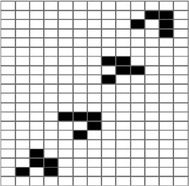
Another important conﬁguration in the Game of Life is the “glider,” a structure with

this initial condition:

111

100

010

The glider represents a local pattern of states of agents that propagates through

the environment diagonally. Note that it is not actually the agents that are moving but

the conﬁguration pattern of states (Fig. 2.2). Apart from being fun to watch, gliders

can be thought of as transmitting information from one part of the grid to another—

information that is relayed from one group of agents to another. Gliders are often

used as essential parts in many more complex conﬁgurations in the Game of Life.

There have even been successful attempts to built entire computing machines purely

from initial conﬁgurations in the Game of Life. In some versions of these conﬁgu-

rations gliders are used as channels to transmit basic units of information between

the parts of the “computer”.

2.2 Start with a glider pattern and use the rules to update it by hand for a few time

steps.

34 2 Agent-Based Modeling

Fig. 2.2 The glider sequence

in the Game of Life. The four

conﬁgurations in the graph

show the sequence a glider

would undergo while moving

diagonally north-eastwards

As far as we are concerned here, the Game of Life is an example of an ABM

that allows for only limited actions and interactions between agents, but can still

produce complex and interesting behaviors. Unfortunately, it is not really useful

beyond being a playground for mathematicians. Nevertheless, it does illustrate the

principles of agent-based modeling—agents with state and rule-based behavior in-

teracting in a structured environment—and shows that even simple interactions can

lead to complex behavior.

The Game of Life also illustrates how ABMs can deal with irreducible hetero-

geneity. All agents in the system are the same, and only differentiated from one

another by their state. Modeling this mathematically would be nearly impossible,

but it is easy to implement as a computer model.

2.3 Check, by hand, the effect of different asynchronous update rules on the glider.

2.4 What happens if two gliders collide?

2.4 Malaria

The Game of Life is one of the simplest possible non-trivial ABMs; it is an interest-

ing world to explore, but it does not have any immediate use as a model of something

real. ABMs as models of some aspects of the real world need to be more advanced

than the Game of Life. In this section we will discuss a somewhat more advanced

(and perhaps practically more useful) example of an ABM, modeling the transmis-

sion of Malaria. Modeling diseases and their spread is an important thing to be able

to do. Models of disease transmission could, at least if they are accurate enough, be

used in a variety of contexts, such as in optimizing responses to emerging epidemics,

or for efﬁcient planning of immunization programs, particularly when resources are

limited.

Particularly in sub-Saharan Africa, Malaria is the single biggest killer, ahead

even of HIV/AIDS. The disease is vector borne, that is, it is transferred from person

2.4 Malaria 35

to person by a secondary agent, the male Anopheles mosquito (the female is not a

vector of Malaria). An infection is transferred both from human to mosquito and

vice versa when Anopheles bites a human.

The dynamics of infection depend on the local interactions between individ-

ual agents, namely the vectors (mosquitoes) and the humans. Both humans and

mosquitoes have a limited range of movement and can only interact when in each

other’s neighborhood. The exact details of how agents move across their available

space—in particular the mosquitoes—could have a major inﬂuence on how fast and

how far Malaria spreads; in this sense there are irreducible interactions. The sys-

tem is also irreducibly heterogeneous, in that some agents are infected some while

are susceptible (that is uninfected). There is a random element to the model in that

the contact between the agent-types is probabilistic. As will become clear below,

this randomness and heterogeneity is, under some conditions, reducible, but irre-

ducible under others. In order to deal with the latter case, an ABM is appropri-

ate.

Let us now leave the preliminaries behind and put into practice what we have

discussed in theory. Our aim is to ﬁnd the simplest non-trivial model of Malaria

that captures the essence of reality. In every modeling enterprise, one should always

try to ﬁnd the simplest model ﬁrst, and only introduce complexities once this sim-

plest model is thoroughly understood. There are many possible choices one can take

when modeling the spread of Malaria. The shape and form of the ﬁnal model will

depend on the particular goals that are to be achieved. Depending on whether they

are predictive, explanatory or exploratory, different requirements need to be put on

the model. Here we do not have any particular purpose in mind, other than demon-

strating how to design ABMs, and we will therefore design the simplest non-trivial

model of the spread of Malaria. Generally, it is a good idea to start in this way, even

when one has a particular purpose in mind. It is a common mistake for modelers to

start designing models that are full of details but are also opaque. Particularly with

ABMs, this danger is ever-present.

As a minimal requirement, an ABM of the transmission dynamics of Malaria will

have to consider at least two types of agents, namely mosquitoes and humans. In a

ﬁrst model, it is best to avoid the complication of distinguishing between female

and male mosquitoes, although for some applications this could become relevant.

Similarly, humans could be differentiated according to age, as different age-groups

will likely have different susceptibilities for the disease and different survival rates.

However, for a ﬁrst attempt it is best to ignore these complicating effects as well. In-

stead, to keep matters simple for an initial model, we reduce the possible states of the

agents to two: either an agent is infected or not. We have to assume that both types of

agents could be either infected or not, and these would be the only two states of the

agents. The difference between human-agents and mosquito-agents is in the details

of the rules that determine how they carry an infection, and for how long they stay

infected. To keep the complexity of the model to a minimum, one would initially

also ignore that agents die (of Malaria or otherwise). This means that there is a ﬁxed

number of agents in the environment. Each agent can be either infected or suscep-

tible. Naturally, we have to assume at least one interaction between mosquitos and

36 2 Agent-Based Modeling

humans, namely cross-infection; the model needs to have some mechanism whereby

mosquitos can infect humans, and vice-versa. Cross-infection can only happen be-

tween neighboring agents (where neighboring refers to some spatial proximity) and

between agents of different type.

A feature that we cannot ignore, even in the initial simple model, is the spa-

tial structure of the population. Agents need to be embedded in an environment.

In the present case the simplest way to represent an environment is to assume a

2-dimensional space, say a square of size L ×L. We will allow the agents to move

in their environment. Static agents seem simpler at ﬁrst, however they are not as

we see below. Moreover, at least the mosquitoes have to be allowed to move. If all

agents were static then no non-trivial disease transmission dynamics could emerge.

Abstracting away all but the most essential details, we end up with a model that

has a ﬁxed number of ageless and immortal agents that move about in their environ-

ment. We summarize here the essentials of our model:

• There are two types of agents: humans and mosquitoes.

• Agents live in a continuous rectangular environment of size L ×L.

• Agents can be in either of two states: infected or susceptible.

• If a mosquito is infected then all humans within a radius b of the mosquito will

become infected.

• If a mosquito is susceptible, and there is an infected human within a radius b of

the mosquito, then the mosquito will become infected.

• Once infected, humans remain infected for R

time steps, mosquitoes will re-

main infected for R

time steps. The actual numbers chosen will be arbitrary, but

should reﬂect the fact that the life span of a mosquito is very short compared to

the likely time a human remains infected.

• All agents move in their world by making a step no larger than s

(humans) or s

(mosquitoes) in a random direction; essentially they take a random position within

a radius of size s

or s

from their present position. Henceforth we will always

keep s

=1; this is a rather arbitrary choice but it simpliﬁes the investigation of

the parameter space by reducing its dimensionality. At the same time, we expect

that it will not make a material difference to the behavior of the model as we

observe it. This rule introduces randomness into the model; the randomness which

will turn out to be irreducible under some conditions.

These choices are of course not unique and have a certain degree of arbitrariness to

them. Following the same principles of simplicity, one could have come up with

a slightly different model. But, for the rest of this section, we now accept this

choice.

Note that this description includes provision for a number of parameters or con-

ﬁguration variables, such as L, b, s

, etc. Identifying appropriate parameter values

is always an important and unavoidable part of the development of an ABM. The

problem with parameters is that they are often not known, but their precise value

could (and typically does) make a huge difference to the behavior of the model.

Finding the correct parameters is, at least within biological modeling, one of the

greatest challenges of any modeling project. In practice one often ﬁnds that a model

2.4 Malaria 37

has more parameters than one anticipated. (We like to refer to this phenomenon as

the law of mushrooming parameters.) One strategy to reduce the number of param-

eters is to leave out interactions, phenomena, and/or details from the model that (i)

require additional parameters and (ii) are perhaps not essential to the particular pur-

poses of the investigation. Keeping the mushrooming under control is not something

that can be done by following the rules given in a book, but requires the sweat and

tears of the modeler who has to go through every aspect of their model and ask,

“Do I really need to include this effect right now?” In general it is a good rule to

commit model details to the executioner, unless their necessity is proved beyond a

reasonable doubt. No mercy should be shown.

The reader will perhaps agree with us that our model of the spread of Malaria is

a bare-bones representation of the real system. Not much can be stripped away from

it without it becoming completely trivial. Still, even this simple model has many

parameters that need to be determined. However, before we start considering these

in more detail, we are going to make a seeming digression and explore the way in

which the mathematics that we have abandoned in favor of computer modeling still

has something left to offer us.

2.4.1 A Digression

One of the problems of computer simulation models in general, and ABMs in par-

ticular, is their lack of transparency. Even when a model is relatively simple, it is

often hard to understand exactly how one would expect the model to behave. This

is particularly true during the early stages of the modeling cycle. Even more so, one

can never be quite sure that the model is actually behaving the way it is meant to.

One source of problems is simply programming bugs. Subtle errors in the code of

the program are often hard to detect, but could make a big difference to the simula-

tion results. In the case of the Game of Life, testing the model is not such a problem.

Once one has tried out a few conﬁgurations with known behavior, one can be rea-

sonably conﬁdent about the correctness of the code. The source of this conﬁdence

is that there is a known reference behavior. The user knows how the model should

behave and can compare the expected behavior with the actually observed one. Un-

fortunately, in most realistic modeling ventures, this will not be true, at least not

across the whole parameter space.

Often, however, it is possible to ﬁnd parts of parameter space where the dynamics

of the model simpliﬁes sufﬁciently to make it amenable to mathematical modeling.

The mathematical model will then provide the reference behavior against which the

correctness of the ABM can be checked.

Apart from the correctness aspect, there is another advantage in making a math-

ematical model: A mathematical formulation will often provide some fundamental

insights into how changes of parameter values impact on the overall behavior of the

model. These insights might not carry over precisely to more general situations in

the parameter space, but they often still provide basic insights that might help shape

the intuition of the modeler.

38 2 Agent-Based Modeling

Let us consider a few key parameters of our Malaria model—those affecting the

ranges of movement of both the humans and the mosquitoes. The simplest case

to consider is that humans move by taking a random position in their world; this

corresponds to s

= L. This particular choice of parameter is perhaps not very re-

alistic with respect to the real system, but it does have the signiﬁcant advantage of

making the model amenable to a mathematical analysis. When all humans choose

a random position in their world, then the spatial conﬁgurations of the agents be-

come unimportant (we keep s

= 1). This limiting case then corresponds to what

we call a perfectly mixed model. In what follows, we will walk through the process

of comparing the model with a mathematical prediction of its behavior.

In the Malaria model with perfect mixing, a mathematical model can be easily

formulated (see [9] for details). If M is the total number of mosquitoes, m the

number of infected vectors, H and h the corresponding variables for the numbers of

humans, R

and R

the times for vectors and humans to recover from an infection,

b the area over which a vector can infect a human during a single time step and W

the total area of the world; then the proportion of infected vectors and humans can

be written as follows:

= 1 −(1 −Q(h))

= 1 −(1 −Q(m))

(2.1)

Here the function Q(x) is given by

Q(x) =1 −exp



−



Note that these equations depend on the density (the number of agents over the size

of the environment) only, and not on the absolute numbers of agents.

Considering these equations, the astute reader will immediately object that the

variables m and h are not dependent on time. This appears to be counter-intuitive.

There surely are parameters that allow overall very high infection levels? Given

such parameters, if we introduced a single infected agent into a healthy population,

it will take some time before high infection levels are reached. It is not clear how

the mathematical model could describe the transient infection levels, given that it

has no representation of time.

This objection is correct, of course. The model does not describe initial condi-

tions at this level of detail and the model does not contain time. Instead, it describes

the long-term or steady state behavior of the model. The steady state of a system,

if it exists at all, is the behavior that is reached when the transient dynamics of the

model has died out. Often, but not always, the steady state behavior is indepen-

dent of the initial state. Certainly in the case of the Malaria model, in the long run

the behavior will be the same, whether we start with a single agent infected or all

of them infected, It is this steady state behavior that the mathematical model (2.1)

describes.

There is one complication: What if we start with no infection at all? According

to the rules of the ABM, independent of the values of b and W an infection can

2.4 Malaria 39

never establish itself unless there is at least one infected agent in the system. This

seems to indicate that, for the special case of m =0 and h =0, initial conditions are

important after all.

A second glance at (2.1) reveals that the mathematical model can indeed repre-

sent this case as well. The reader can easily convince herself that the case h =0 and

m = 0 always solves the set of equations, independent of the values of b and W .

This tells us that, for some parameter sets, the model has two solutions:

• The case where a certain fraction of the mosquitoes and the humans are infected.

This solution, if it exists, will always be observed in the model, unless we start

with no infected agents at all.

• The other case is possible over the entire space of parameters, and describes the

situation where there is no infected agent in the model.

Whether or not there are two or just one solution to the model depends on the

parameters. If there are two solutions then the solution corresponding to no infection

at all (the “trivial solution”) is, in a technical sense, unstable. In practice this means

that the introduction of a single infected agent (human or mosquito) is sufﬁcient

for the system to approach the non-trivial solution. In this case, the disease would

establish itself once introduced.

In the part of the parameter space that admits only one solution, the long-term

behavior will always be the trivial behavior. No matter how the initial state is chosen,

whether there are many infected agents, or no infected agents, Malaria will never be

sustained in the system. For the particular mathematical model in (2.1) it is possible

to derive the range of parameters for which there is only one solution. We will not

derive the formula here, but be content to state the result. The reader interested in

exploring the details of the model is referred to the primary literature [9]. The model

in (2.1) has two solutions only if the following condition is fulﬁlled:

√

MHR

(2.2)

Essentially, this means that the area b over which the mosquitoes can infect humans

within a single time step needs to be sufﬁciently large in relation to the overall size of

the system (W ) so that an infection can establish itself. What counts as “sufﬁciently

large” depends on the total numbers of mosquitoes and humans and for how long

they remain infected once they are bitten by a mosquito.

2.4.2 Stochastic Systems

There is one additional qualiﬁcation to the validity of (2.2) that is of more general

importance in modeling. Strictly speaking, the condition is only valid in the case

of a deterministic system. The concept of a deterministic system is perhaps best

understood by explaining what is not a deterministic system.

Assume in our Malaria model a set of parameters that allows a non-trivial so-

lution. Assume further that we choose our initial conditions such that all human

40 2 Agent-Based Modeling

agents are susceptible, and only a single mosquito is initially infected. According

to the preceding discussion we would now expect the infection to take hold in the

system and, after some time, we should observe the non-trivial steady state infection

levels as predicted by the model (2.1).

In the model, this is not necessarily what we will observe. Remember that, in the

case of perfect mixing, both mosquitoes and humans take up random positions at

every time step. It is not impossible that, by some ﬂuke event, at the beginning of

the simulation the single infected agent is in an area where there are no other human

agents at all. This probability can be easily calculated from the Poisson distribu-

tion:

P(no human) =exp



−



(2.3)

Here Hb/W is the average number of human agents one would expect within

the bite area of the mosquito. Remember now that the infection of a single agent

lasts for R

or R

time steps. In the case we are considering here, the prob-

ability that an infection is introduced by a single mosquito is not passed on

is then given by P

. Depending on the values of the parameters, this prob-

ability could be very small, but it is never vanishing. Simple stochastic ﬂuc-

tuations can wipe out an infection, particularly when the number of infected

agents is low. Hence, the behavior predicted by the mathematical models (2.1)

and (2.2) might not always be correct, because of stochastic ﬂuctuations in the sys-

tem.

There is another—probably more important—sense in which our Malaria model

is non-deterministic. When simulating the model, one will typically ﬁnd that the

actually observed number of infected agents is not exactly equal to the predicted

number, but will be a bit higher or lower than the predicted number. The reason for

this is that the mathematical model only tells us about the mean number of agents

in the long run. Stochastic ﬂuctuations ensure that actual infection levels will vary

somewhat over time, and either be a bit higher or a bit lower than the mean. The

source of these ﬂuctuations is the randomness in the rules of the system, particularly

the randomness in contact between humans and mosquitos. A good comparison is

a coin ﬂipping experiment. If one ﬂips a coin 10 times then, on average, one would

expect to see “head” 5 times. In an actual experiment this could happen, but one

will often observe that the number of heads deviates from this “mean.” In essence,

this is the same type of stochastic ﬂuctuation that leads to the deviation from the

calculated mean behavior in the Malaria model.

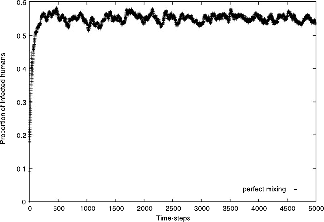
Figure 2.3 shows an example of a simulation of the Malaria model. The particular

graph plots the proportion of infected agents at every time step. The simulation

shown in the ﬁgure starts with no humans being infected. In order to avoid the

trivial solution, we start with half of the mosquito population being infected. In the

perfect mixing case, the population of infected agents rises initially, until it reaches

its expected steady-state behavior. After this transient period, the infection level of

the humans stays close to the theoretical steady state value, as calculated from the

model (2.1). The level of infection never quite settles on the expected behavior,

which is another manifestation of the stochastic ﬂuctuations.

2.4 Malaria 41

Fig. 2.3 An example of the time-evolution of the proportion of infected humans in the Malaria

model when perfect mixing is assumed. We start with a half of the mosquitos infected. After a

rapid initial increase in the infection levels, the system ﬁnds its steady-state and the infection level

ﬂuctuates around some long-term mean value

Stochastic ﬂuctuations are often referred to as noise. Just how much noise there

is in this system depends on the size of the population. In practical modeling ap-

plications it is often necessary to reduce the noise of models. In these situations

it will be useful to scale the model. By this we mean a change of the parameters

that leaves the fundamental properties of the model unchanged but, in this particular

case, increases the number of agents in the system. What counts as a “fundamen-

tal property” is problem dependent. In our case here, the fundamental variable we

are interested in is infection level, so the fraction of agents that carry the infec-

tion.

If we attempted to reduce the noise by simply changing the number of humans

in the model, we might reduce the noise, but we also change the expected levels

of infection by changing the density of humans in their “world” and the number

of humans in relation to mosquitoes; this would not be scaling. In order for the

properties of the model to remain the same, we also need to change the size of the

world and the number of mosquitoes such that the scaled up model has the same

density of mosquitoes and agents as the original model.

The expected behavior, as calculated from (2.1), will be the same at all scales,

but the relative ﬂuctuations around the expected behavior will be smaller the greater

the number of agents; note that the mathematical model itself is formulated in terms

of agent densities only. Only in the limit of an inﬁnitely large population will the

expected steady state behavior equal the observed one. The effect of scaling on noise

Barnes D.J., Chu D. Introduction to Modeling for Biosciences

Подождите немного. Документ загружается.