Atkinson K. An Introduction to Numerical Analysis
Подождите немного. Документ загружается.

PIECEWISE POLYNOMIAL INTERPOLATION
167
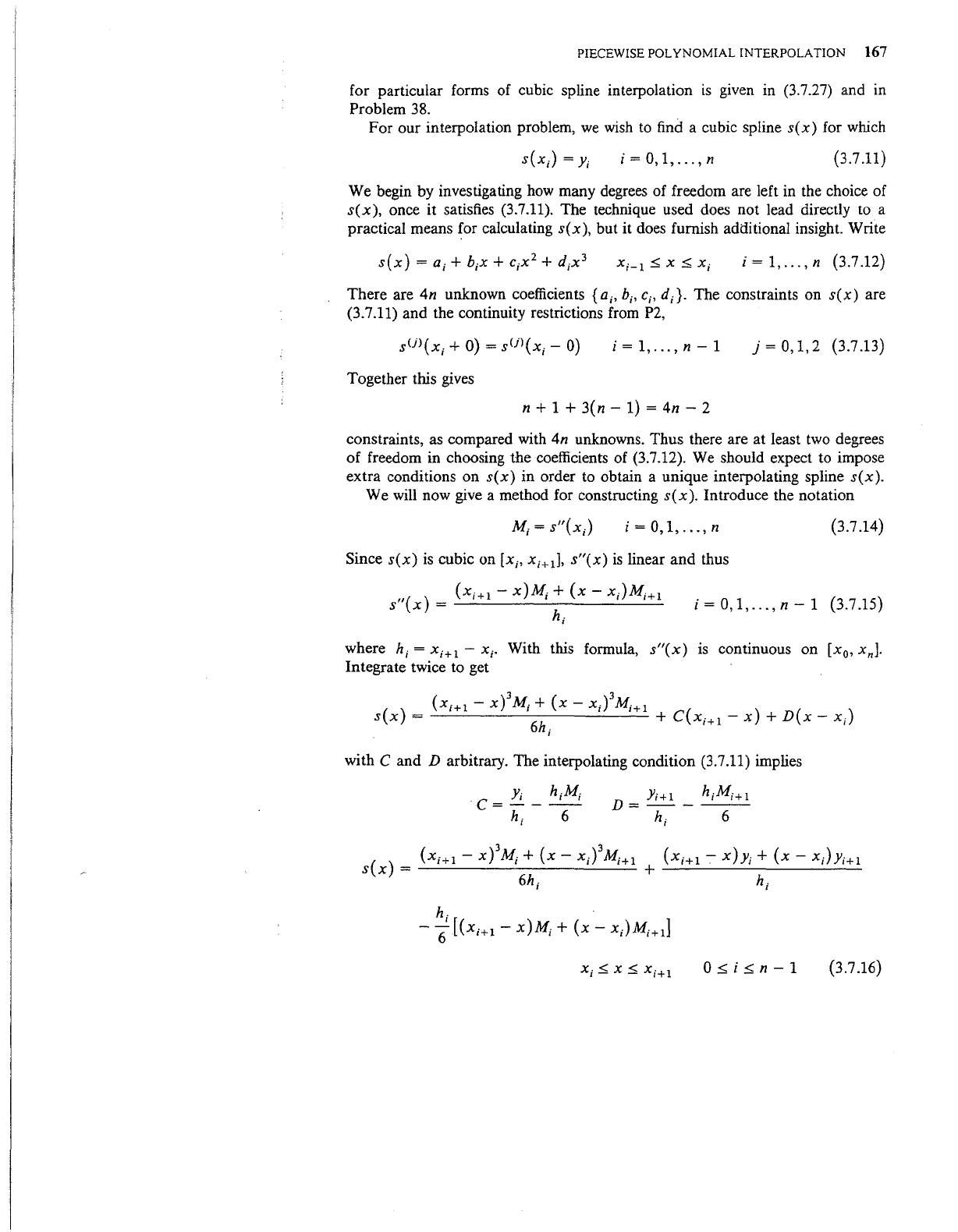
for particular forms of cubic spline interpolation
is
given
in
(3.7.27) and
in
Problem
38.
For our interpolation problem,
we
wish
to
find a cubic spline
s(x)
for which
i=0,1,
...
,n
(3.7.11)
We begin by investigating
how
many degrees of freedom are left
in
the choice of
s(x),
once it satisfies (3.7.11). The technique used does not lead directly to a
practical means for calculating
s(x),
but it does furnish additional insight. Write
i = 1,
...
, n (3.7.12)
There are
4n unknown coefficients {a;,
b;.
c;.
d;}. The constraints on
s(x)
are
(3.7.11) and the continuity restrictions from
P2,
i=1,
...
,n-1
j=0,1,2
(3.7.13)
Together this gives
n
+ 1 +
3(n-
1) = 4n - 2
constraints, as compared with 4n unknowns. Thus there are at least two degrees
of
freedom in choosing the coefficients of (3.7.12).
We
should expect to impose
extra conditions on
s(x)
in order to obtain a unique interpolating spline
s(x
).
We
will
now give a method for constructing
s(x).
Introduce the notation
i=0,1,
...
,n
(3.7 .14)
Since
s(x)
is
cubic on [x;,
X;+d,
s"(x)
is
linear
and
thus
(x;+I-
x)M;
+
(x-
x;)Mi+I
s"(x)
=
---------
h;
i=0,1,
...
,n-1
(3.7.15)
where
h; =
X;+I-
X;.
With this formula,
s"(x)
is
continuous on
[x
0
,
xnl·
Integrate twice to get
(xi+ I - x )
3
M;+
(x-
x;)
3
Mi+
1
s(x)
=
6
h.
+
C(xi+I-
x)
+
D(x-
x;)
I
with C and D arbitrary. The interpolating condition (3.7.11) implies
y. h .M.
c = ..}_-
_,_,
h; 6
O~i~n-1
(3.7 .16)
168
INTERPOLATION
THEORY
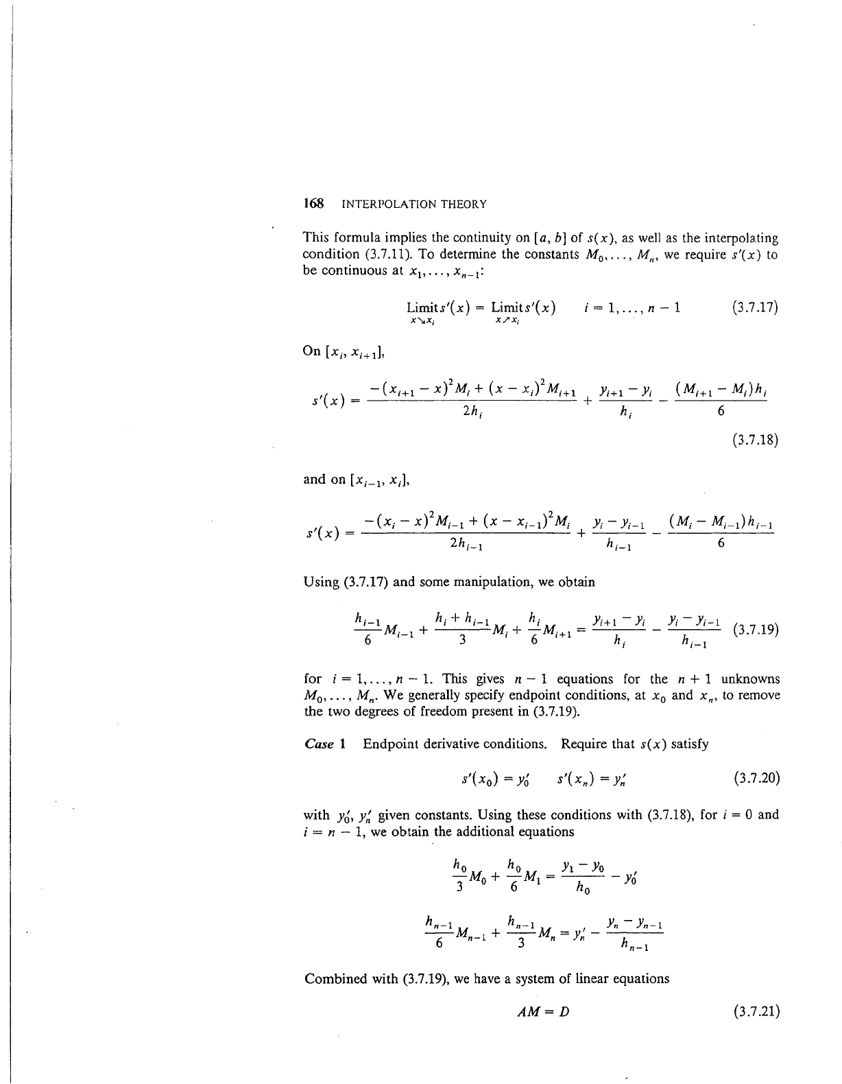
This formula implies the continuity on [a,
b]
of
s(x),
as well
as
the interpola.ting
condition (3.7.11).
To
determine the constants M
0
,
•..
,
Mn,
we
require
s'(x)
to
be
continuous
at
x
1
,
•••
,
xn-t:
Lirnits'(x)
=
Lirnits'(x)
i=1,
...
,n-1
(3.7.17)
X'\.X;
X/'Xl
-
(Xi+
1 -
X)
2
M;
+
(X
- X y
M;
+ 1 +
Y;
+ 1 -
Y;
s'(x)
=
-----------
2h; h;
and
on
[x;_
1
,
X;],
Using
(3.7.17)
and
some manipulation,
we
obtain
(M;+t-
M;)h;
6
(3.7 .18)
(M;-
M;-t)h;-t
6
Y;-
Y;-t
hi-1
(3.7.19)
for
i = 1,
...
, n -
1.
This gives n - 1 equations for the n + 1 unknowns
M
0
,
•••
, Mn.
We
generally specify endpoint conditions, at x
0
and xn, to remove
the two degrees
of
freedom present in (3.7.19).
Case
1
Endpoint
derivative conditions. Require
that
s(x)
satisfy
'( ) - ,
s
Xo
-Yo
(3.7
.20)
with y
0
,
y;
given constants. Using these conditions with (3.7.18), for i = 0 and
i = n - 1, we obtain the additional equations
hn-1 hn-1
1
Yn-
Yn-1
-6-Mn-1
+ -
3
-Mn
= Y -
n
hn-1
Combined
with (3.7.19),
we
have a system
of
linear equations
AM=D
(3.7 .21)
PIECEWISE POLYNOMIAL INTERPOLATION 169
with
DT
_
[Y1
-Yo
_ ,
Y1-
Y1
- h Yo, h
0 1
Y1-
Yo
ho
, ... ,
ho
-
3
ho
-
6
A=
0
0
0
Yn-
Yn-l
hn-l
ho
-
6
ho +
hr
3
hl
-
6
Yn-l-
Yn-1
1
Yn-
Yn-l
.]
-
y-
hn-2
' n
hn-l
0
0
0
hl
-
6
hl
+ h1
3
hn-1
hn-1
+
hn-l
hn-l
6
3
6
hn-l
hn-l
6 3
(3.7 .22)
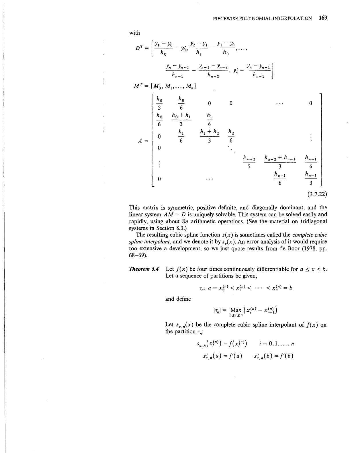
This matrix
is
symmetric, positive definite, and diagonally dominant, and the
linear system
AM
= D
is
uniquely solvable. This system can be solved easily and
rapidly, using about
8n
arithmetic operations. (See the material on tridiagonal
systems in Section
8.3.)
The resulting cubic spline function
s(x)
is
sometimes called the complete cubic
spline interpolant,
and
we
denote it by
s/x).
An error analysis of it would require
too extensive a development, so
we
just quote results from de Boor (1978, pp.
68-69).
Theorem 3.4 Let
f(x)
be four times continuously differentiable for a
::::;;
x::::;; b.
Let a sequence of partitions
be
given,
and define
I
T I = Max
(x(n)
-
x(n))
n 1
1-1
1s;is;n
Let
sc,n(x)
be the complete cubic spline interpolant
of
f(x)
on
the partition
Tn:
sc,n(xfn>)=J(xfnl)
i=O,l,
...
,n
s:.n(a)
=f'(a)
s:.n(b)
=f'(b)
170
INTERPOLATION THEORY
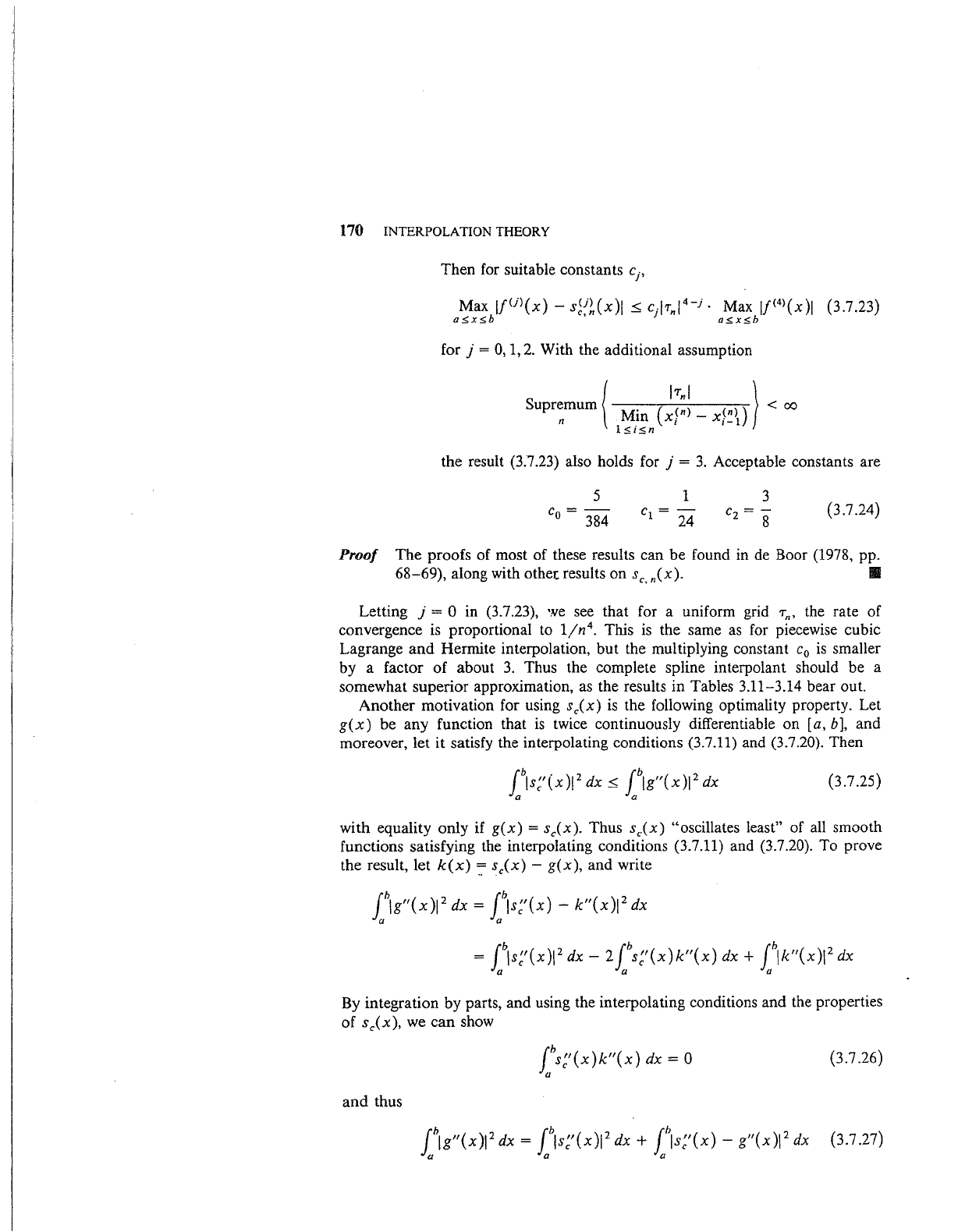
Then for suitable constants c
1
,
Max
ifUl(x)-
s~i~(x)l
~
c.Jrni
4
-J
·
Max
lf<
4
>(x)l
(3.7.23)
a5,x5,b
'
1
as,xs,b
for j =
0,
1,
2.
With the additional assumption
(
lrnl
)
Supremum . (
(n)
_
(n))
<
oo
n
Mm
X;
X;-1
ls,is,n
the result (3.7.23) also holds for j =
3.
Acceptable constants are
5 1
3
c
=-
0 384
c
=-
1
24
Cz
=-
8
(3.7.24)
Proof
The
proofs of most of these results can
be
found in de Boor (1978, pp.
68-69),
along with
othetresults
on
sc.n(x).
Ill
Letting j = 0 in (3.7.23),
'.'le
see that for a uniform grid r", the rate of
convergence is proportional to
1jn
4
•
This is the same as for piecewise cubic
Lagrange
and
Hermite interpolation,
but
the multiplying constant c
0
is
smaller
by a factor
of
about
3.
Thus the complete spline interpolant should be a
somewhat superior approximation, as the results
in
Tables 3.11-3.14 bear out.
Another
motivation for using sc(x)
is
the following optimality property. Let
g(x)
be
any
function that
is
twice continuously differentiable
on
[a,
b],
and
moreover, let it satisfy the interpolating conditions (3.7.11) and (3.7.20). Then
(3.7.25)
with equality only if
g(x)
= sc(x). Thus sc(x) "oscillates least"
of
all smooth
functions satisfying the interpolating conditions (3.7.11) and (3.7.20). To prove
the result, let
k(x)
~
sc(x)-
g(x),
and write
jblg"(x)IZ dx =
fis~'(x)-
k"(x)l
2
dx
a a
=
fis~'(x)l
2
dx-
2jbs~'(x)k"(x)
dx
+
fik"(x)l
2
dx
a a a
By integration by parts,
and
using the interpolating conditions and the properties
of
sc(x), we
can
show
ts~'(x)k"(x)
dx
= 0
a
(3.7.26)
and
thus
jblg"(x)J
2
dx
=
fis~'(x)J
2
dx
+
fis~'(x)-
g"(x)i
2
dx
(3.7.27)
a a a
PIECEWISE
POLYNOMIAL
INTERPOLATION
171
This proves (3.7.25). Equality
in
(3.7.25) occurs only if
s;'(x)-
g"(x)
= 0 on
[a,b], or equivalently
sc(x)-
g(x)
is
linear. The interpolating conditions then
imply
s"(x)
-
g(x)
=
0.
We
leave a further discussion of this topic to Problem
38.
Case 2 The "not-a-knot" condition. When the derivative values
f'(a)
and
f'(b)
are not available,
we
need other end conditions on
s(x)
in
order
to
complete the system of equations (3.7.19). This
is
accomplished by requiring
s<
3
>(x) to be continuous at x
1
and
xn-t·
This
is
equivalent to requiring that
s(x)
be a cubic spline function with knots { x
0
,
x
2
,
x
3
,
..•
, xn_
2
,
~n
}, while still
requiring interpolation at
all
node points in
{x
0
,x
1
,x
2
,
...
,xn-l•xn}·
This
reduces system
(3.7.19)
ton-
3 equations, and the interpolation at x
1
and xn_
1
introduces two new equations
(we
leave their derivation
to
Problem
34).
Again
we
obtain a tridiagonal linear system
AM=
D, although the matrix A does not
possess some of the nice properties of that in
(3.7.22). The resulting spline
function will be denoted here by
snk(x), with the subscript indicating the
"not-a-knot" condition. A convergence analysis can be given for snk(x), similar
to that given
in
Theorem 3.4. For a discussion of this, see de Boor (1978,
p.
211),
(1985).
There are other ways of introducing endpoint conditions when
f'(a)
and
f'(
b)
are unknown. A discussion of some of these can be found in de Boor (1978,
p. 56). However, the preceding scheme
is
the simplest to apply, and it
is
widely
used. In special cases, there are simpler endpoint conditions that can be used
than those discussed here, and
we
take
up
one of these in Problem 38. In general,
however, the preceding type of endpoint conditions are needed in order to
preserve the rates of convergence given
in
Theorem 3.4.
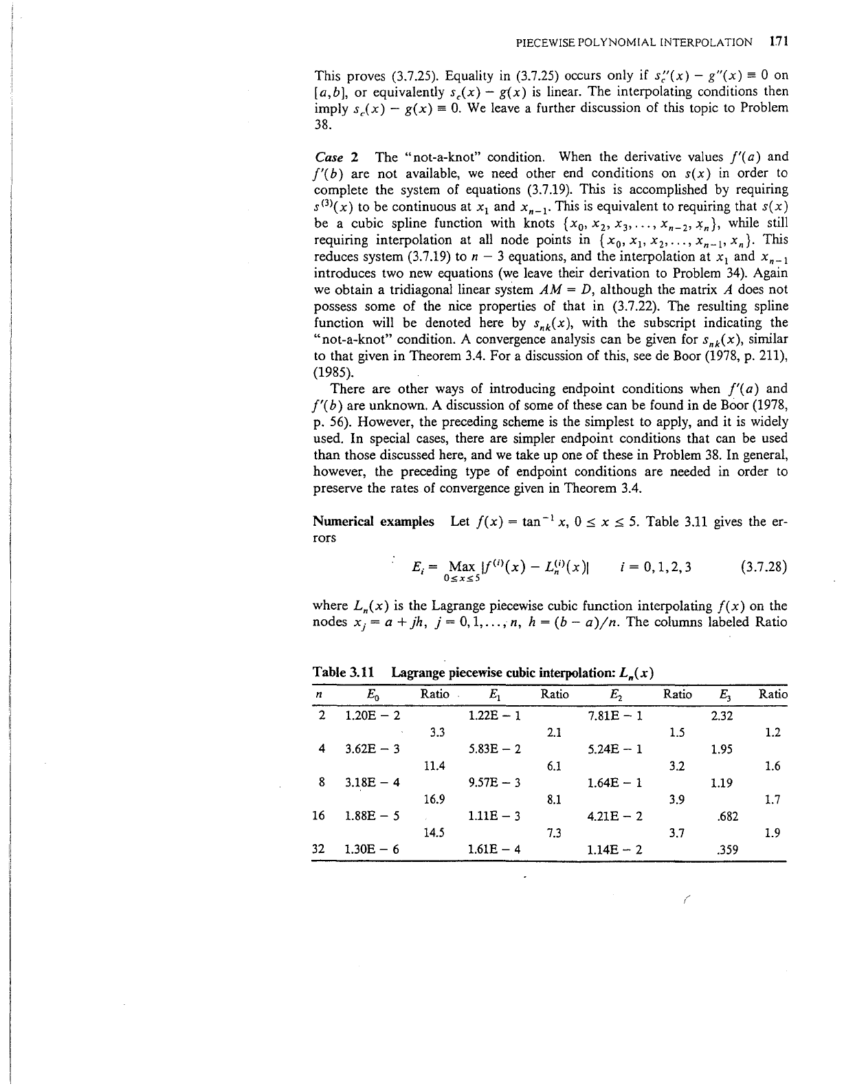
Numerical examples Let
f(x)
=
tan-
1
x, 0
~
x
~
5.
Table 3.11
gives
the er-
rors
E;
= Max
IJU>(
x)
-
L~;>(
x
)I
0:Sx:S5
i = 0,
1,2,3
(3.7.28)
where
Ln(x)
is the Lagrange piecewise cubic function interpolating
f(x)
on the
nodes
xj
=a+
jh,
j =
0,
1,
...
, n, h =
(b-
a)jn.
The columns labeled Ratio
Table 3.11
Lagrange piecewise cubic interpolation:
Ln(x)
n
Eo
Ratio
Et
Ratio
£2
Ratio
E3
Ratio
2
1.20E-
2
1.22E-
1
7.81E-
1
2.32
3.3
2.1
1.5
1.2
4
3.62E-
3
5.83E-
2
5.24E-
1
1.95
11.4
6.1
3.2
1.6
8
3.18E-
4
9.57E-
3
1.64E-
1
1.19
16.9
8.1
3.9
1.7
16
1.88E-
5
l.llE-
3
4.21E-
2
.682
14.5
7.3
3.7
1.9
32
1.30E-
6
1.61E-
4
1.14E-
2
.359
/
I
172
INTER
PO LA
TION
THEORY
Table 3.12
Hermite piecewise cubic interpolation:
Q
n(
X)
n
Eo
Ratio
Ei
Ratio
E2
Ratio
E3
Ratio
3
2.64E-
2
5.18E-
2
4.92E-
1
2.06
5.6
3.0
2.3
1.5
6
4.73E-
3
1.74E-
2
2.14E-
1
1.33
16.0
8.0
3.6
1.5
12
2.95E-
4
2.17E-
3
5.91E-
2
.891
13.1
6.7
3.6
1.9
24
2.26E-
5
3.25E-
4
1.66E-
2
.475
16.0
8.0
4.0
2.0
48
1.41E-
6
4.06E-
5
4.18E-
3
.241
give the
rate
of
decrease in the error when n
is
doubled.
Note
that
the rate of
convergence for
L~i)
to
[U>
is
proportional to h
4
-;,
i = 0,
1,
2,
3.
This can be
rigorously proved, and an indication
of
the proof is given in Problem 32.
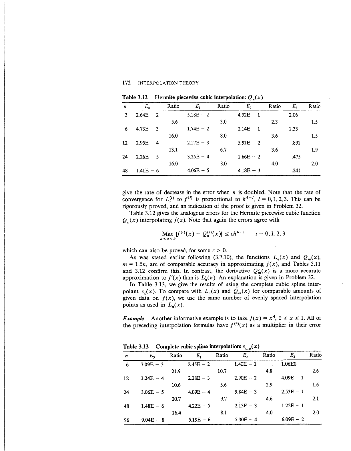
Table 3.12 gives the analogous errors for the Hermite piecewise cubic function
Qn(x)
interpolating
f(x).
Note that again the errors agree with
Max
IJU>(x)-
Q~il(x)l
:::;;
ch
4
-;
a;5;xs;b
i =
0,
1,
2, 3
which can also
be
proved, for some c > 0.
As was
stated
earlier following (3.7.10), the functions
Ln(x)
and
Qm(x),
m =
l.5n,
are
of
comparable accuracy in approximating
f(x),
and Tables
3.11
and
3.12 confirm this.
In
contrast, ·the derivative
Q:,(x)
is
a more accurate
approximation to
f'(x)
than
is
L~(n).
An explanation is given in Problem 32.
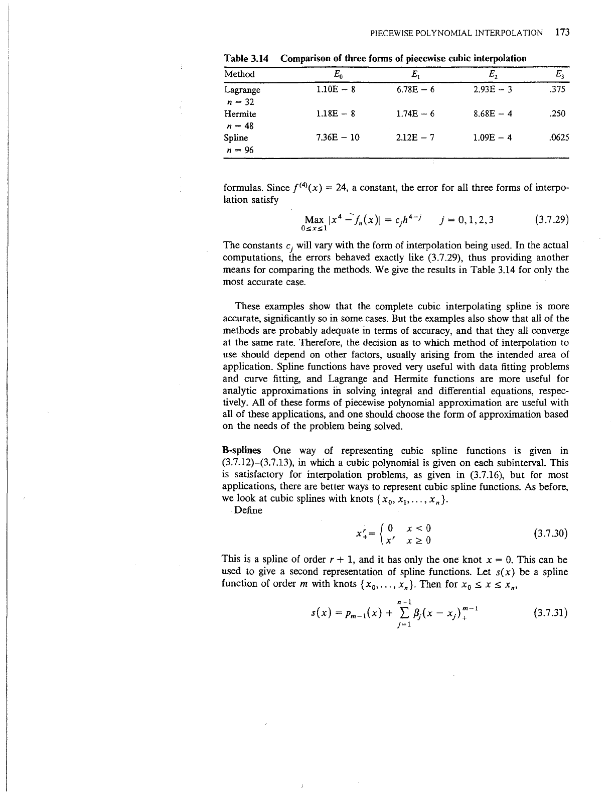
In
Table
3.13, we give the results
of
using the complete cubic spline inter-
polant
sc(x).
To
compare with
Ln(x)
and
Qm(x)
for comparable amounts
of
given
data
on
f(x),
we use the same number
of
evenly spaced interpolation
points as used in
Ln(x).
Example
Another
informative example is to take
f(x)
=
x\
0:::;;
x:::;;
1.
All of
the preceding interpolation formulas have
[<
4
>(x)
as a multiplier in their error
Table
3.13
Complete cubic spline interpolation:
sc,ix)
n
Eo
Ratio
Ei
Ratio
E2
Ratio
E3
Ratio
6
7.09E-
3
2.45E-
2
1.40E-
1
1.06EO
21.9
10.7
4.8
2.6
12
3.24E-
4
2.28E-
3
2.90E-
2
4.09E-
1
10.6
5.6
2.9
1.6
24
3.06E-
5
4.09E-
4
9.84E-
3
2.53E-
1
20.7
9.7
4.6
2.1
48
1.48E-
6
4.22E-
5
2.13E-
3
1.22E-
1
16.4
8.1
4.0
2.0
96
9.04E-
8
5.19E-
6
5.30E-
4
6.09E-
2
PIECEWISE
POLYNOMIAL
INTER
PO
LA TION
173
Table 3.14
Comparison of three forms of piecewise cubic interpolation
Method
Eo
£1
Ez
£3
Lagrange
l.lOE-
8
6.78E-
6
2.93E-
3
.375
n =
32
Hermite
l.18E-
8
1.74E-
6
8.68E-
4 .250
n =
48
Spline
7.36E-
10
2.12E-
7
1.09E-
4
.0625
n =
96
formulas. Since
J<
4
>(x) = 24, a constant, the error for all three forms of interpo-
lation satisfy
j =
0,1,2,3
(3.7.29)
The
constants
cj
will vary with the form of interpolation being used.
In
the actual
computations, the errors behaved exactly like (3.7.29), thus providing another
means for comparing the methods. We
give
the results in Table 3.14 for only the
most accurate case.
These examples show
that
the complete cubic interpolating spline
is
more
accurate, significantly so in some cases. But the examples also show
that
all
of
the
methods are probably adequate in terms of accuracy,
and
that
they all converge
at the same rate. Therefore, the decision
as
to which method of interpolation to
use should depend on other factors, usually arising from the intended area
of
application. Spline functions have proved very useful with
data
fitting problems
and
curve fitting, and Lagrange and Hermite functions are more useful for
analytic approximations
in solving integral and differential equations, respec-
tively. All
of
these forms
of
piecewise polynomial approximation are useful with
all
of
these applications, and
one
should choose the form
of
approximation based
on
the needs
of
the problem being solved.
B-splines
One
way of representing cubic spline functions is given in
(3.7.12)-(3.7.13), in which a cubic polynomial
is
given
on
each subinterval. This
is satisfactory for interpolation problems, as given in
(3.7.16),
but
for most
applications, there are better ways to represent cubic spline functions. As before,
we look at cubic splines with knots {
x
0
,
x
1
,
...
, xn } .
. Define
;
{0
x<O
X -
+-
x'
x
:2:.
0
{3.7 .30)
This is a spline
of
order r + 1, and it has only the
one
knot x =
0.
This can be
used to give a second representation of spline functions. Let
s(x)
be
a spline
function
of
order m with knots { x
0
,
•••
,
xn
}.
Then for x
0
~
x
~
xn,
n-1
s(x)
= Pm-l(x) + L /3;·(x-
xj):-l
j=l
(3.7 .31)
174 INTERPOL.' TION THEORY
with Pm-
1
(x)
a uniquely chosen polynomial
of
degree.::;;
m-
1
and
{3
1
,
•••
,
{3,_
1
uniquely
determined
coefficients.
The
proof
of this result
is
left as Problem 37.
There
are
several unsatisfactory features to this representation when applying it
to
the
solution
of
other problems.
The
most serious problem
is
that
it often leads
to
numerical
schemes
that
are ill-conditioned.
For
this reason, we
introduce
another
numerical
representation
of
s(x),
one
that
is much better in its numerical
properties.
To
simplify the presentation, we consider only cubic splines.
We
begin
by
augmenting the knots {
Xo,
...
, X
n}.
Choose additional
knots
(3.7.32)
in
some
arbitrary
manner.
For
i = -
3,
-
2,
...
, n -
1,
define
(3.7.33)
a
fourth-order
divided difference
of
fxCt)
=
(t-
x)~
(3.7 .34)
The
function
B;(x)
is called a B-spline, which is
short
for basic spline function.
As
an
alternative
to (3.7.33), apply
the
formula (3.2.5) for divided differences,
obtaining
i+4
(xi-
x)~
B;(x)
=
(x;+
4
-
xJ
~-
"o/-'(x
.)
;-r
r J
This
shows
B;(x)
is a cubic spline with knots
X;,
...
,
X;+
4
•
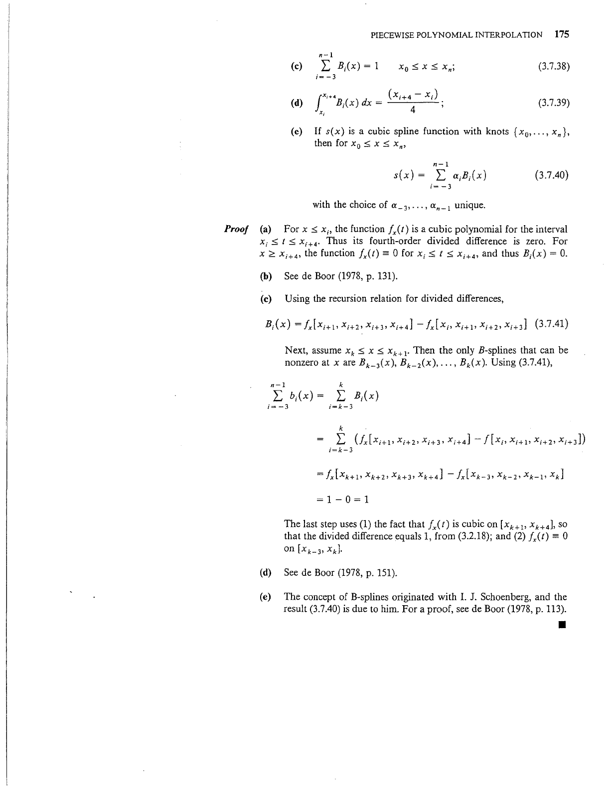
A
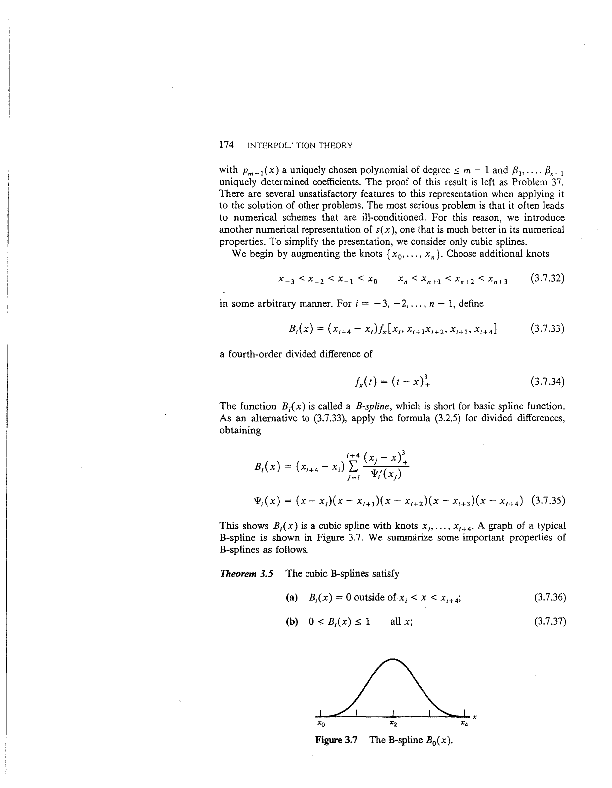
graph
of
a typical
B-spline is
shown
in Figure 3.7.
We
summarize some
important
properties
of
B-splines
as
follows.
Theorem 3.5
The
cubic B-splines satisfy
(a)
B;(x)
= 0 outside
ofx;
< x <
X;+
4
;
(b) O.::;;B;(x).::;;l
all x;
Figure 3.7
The
B-spline B
0
(x).
(3.7.36)
(3.7.37)
PIECEWISE POLYNOMIAL INTERPOLATION
175
n-1
(c)
1:
B;(x) = 1
Xo
~X~
Xn;
(3.7.38)
i=
-3
fxi+4
(xi+4-
x;)
(d)
B;(x) dx =
4
(3.7.39)
X;
(e)
If
s(x)
is
a cubic spline function with knots
{x
0
,
...
, xn},
then for
Xo
~
X
~
Xn,
n-1
s(x)
= L
a;B;(x)
(3.7 .40)
i=
-3
with the choice of
a_
3
,
.••
,
an-l
unique.
Proof
(a)
For
x
~
X;,
the function
fAt)
is a
cubic
polynomial for the interval
X;
~
t
~
X;+
4
•
Thus its fourth-order divided difference
is
zero.
For
x
~
X;+
4
, the function fxCt) = 0 for
X;~
t
~
X;+
4
, and thus
B;(x)
=
0.
(b)
See de Boor (1978, p. 131).
(c) Using the recursion relation for divided differences,
Next, assume
xk
~
x
~
xk+
1
.
Then
the
only B-splines that can be
nonzero at
x are Bk_
3
(x),
Bk_
2
(x),
...
,
Bk(x).
Using (3.7.41),
n-1
k
L b;(x) = L
B;(x)
i=
-3
i=k-3
k
L
(fx[xi+l•
xi+2•
xi+3•
xi+4]-
f[x;,
Xi+l•
xi+2•
xi+3])
i=k-3
=1-0=1
The
last step uses (1) the fact that
fx(t)
is
cubic on [xk+l•
xk+
4
],
so
that the divided difference equals
1,
from (3.2.18); and (2)
fx(t)
= 0
on [xk_
3
,
xd.
(d) See de Boor (1978, p. 151).
(e) The concept of B-splines originated with
I.
J. Schoenberg, and the
result (3.7.40)
is
due to him.
For
a proof, see de Boor (1978, p. 113) .
•
176 INTERPOLATION THEORY
Because of (3.7.36), the sum
in
(3.7.40) involves at most four nonzero terms.
For
xk
::::;
x <
xk+l•
k
s(x)=
I:
o:;Br(x)
(3.7.42)
i-k-3
In addition, using (3.7.37) and (3.7.38),
showing
that
the value of s(
x)
_is
bounded_by coefficients for B-splines near to x.
I~
this sense, (3.7.40)
is
a local representation of
s(x),
at each x E
[x
0
,
xnl·
A more general treatment of B-splines
is
given in de Boor (1978, chaps. 9-11),
along with further properties omitted here. Programs are also given for comput-
ing with B-splines.
An important generalization of splines arises when
the knots are allowed
to
coalesce. In particular, let some of the nodes
in
(3.7.33) become coincident. Then,
so as long as
X;
<
X;+4•
th~
function
B;(x)
will
be a cubic piecewise polynomial.
Letting two knots coalesce
will
reduce from
two
to one the number of continuous
derivatives at the multiple knot. Letting three knots coalesce will mean that
B;(x)
will only be continuous. Doing this, (3.7.40) becomes a representation for
all cubic piecewise polynomials. In this scheme of things, all piecewise poly-
nomial functions are spline functions, and
vice
versa. This
is
fully explored in
de Boor
(1978).
3.8 Trigonometric Interpolation
An extremely important class of functions are the periodic functions. A function
f(t)
is
said to
be
periodic with period T if
f(t
+
T)
=
f(t)
-oo<t<oo
.
and this
is
not
to be true for any smaller positive value of
T.
The best known
periodic functions are the trigonometric functions.
Periodic functions occur
widely
in applications, and this motivates our consideration of interpolation
suitable for
data
derived from such functions. In addition,
we
use this topic to
introduce the fast Fourier transform
(FFr),
which
is
used
in
solving many
problems that involve data from periodic functions.
By
suitably scaling the independent variable, it
is
always possible to let
T =
2'1T
be the period:
/(
t +
2'1T)
=
/(
t)
-oo<t<oo
We approximate such functions
f(t)
by using trigonometric polynomials,
n
p,(t) = a
0
+
I:
a
1
cos(jt)
+ b
1
sin(jt)
j-1
(3.8.1)
(3.8.2)
