Atkinson K. An Introduction to Numerical Analysis
Подождите немного. Документ загружается.

FURTHER RESULTS ON INTERPOLATION ERROR
157
.Y
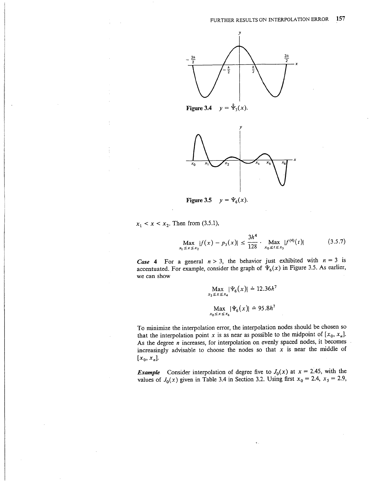
Figure 3.4 y =
~
3
(x).
y
Figure3.5 y =
'1'
6
(x).
x
1
< x < x
2
•
Then from (3.5.1),
(3.5.7)
Case 4
For
a general n >
3,
the behavior
just
exhibited with n = 3 is
accentuated.
For
example, consider the graph of
'¥
6
(x)
in Figure 3.5. As earlier,
we can show
Max l'l'
6
(x)l
~
12.36h
7
x
2
.sx:s;x
4
Max l'l'
6
(x)l
~
95.8h
7
x
0
.:Sx::::;
x
6
To
minimize the interpolation error, the interpolation nodes should
be
chosen so
that the interpolation point x
is
as near
as
possible to the midpoint
of
[x
0
,
xnl·
As the degree n increases, for interpolation
on
evenly spaced nodes, it becomes
increasingly advisable to choose the nodes so that x
is
near the middle of
[xo, xnl·
Example Consider interpolation of degree
five
to
J
0
(x)
at x =
i45,
with the
values of J
0
(x)
given in Table 3.4 in Section 3.2. Using first x
0
= 2.4, x
5
= 2.9,
158 INTERPOLATION THEORY
we
obtain
p
5
(2.45) = -0.232267384
Error=
-4.9
X
10-
9
Second, use x
0
= 2.2, x
5
= 2.7. Then
p
5
(2.45) = -0.232267423 Error = 1.0 X
10-
9
The error
is
about
five
times smaller, due to positioning x near the middle of
[xo,
Xsl·
The tables in Abramowitz and Stegun (1964) are given to many significant
digits, and the grid spacing
h
is
not correspondingly small. Consequently,
high~degree
interpolation must be
~sed.
Although this results
in
more work for
the user of the tables, it allows the table to be compacted into a much smaller
space; more tables of more functions can then be included in the volume. When
interpolating with these tables and using high-degree interpolation, the nodes
should be so chosen that
x
is
near
(x
0
+
x,)/2,
if possible.
The approximation problem In using a computer,
we
generally prefer to store
an analytic approximation to a function rather than a table of values from which
we
interpolate. Consider approximating a given function
f(x)
on a given interval
[a,
b J by using interpolating polynomials. In particular, consider the polynomial
p,(x)
produced by interpolating
f(x)
on an evenly spaced subdivision of [a,
bJ.
For
each n
~
1,
define h =
(b-
a)jn,
x
1
= a + jh, j =
0,
1,
...
, n. Let
p,(x)
be the polynomial interpolating to
f(x)
at x
0
,
•..
, xn- Then
we
ask whether
Max
lf(x)-
p,(x)l
as.xs;,b
(3.5.8)
tend to zero as n
~
oo?
The answer
is
not necessarily. For many functions, for
example,
ex
on
[0,
1],
the error in (3.5.8) does converge to zero as n
~
oo
(see
Problem
24). But there are other functions, that are quite
well
behaved, for which
convergence does not occur.
The most famous example of failure to converge
is
one due to Carl Runge. Let
1
f(x)
= 1
+x2
-5s;xs;5
(3.5.9)
In
Isaacson and Keller (1966, pp. 275-279), it
is
shown that for any
3.64 < lxl < 5,
Supremum If(
x)
-
p,
( x
)I
=
oo
and k
~
0
(3.5.10)
n"<!:.k
HERMITE INTERPOLATION 159
y
y =
P,o(x)
-5
5
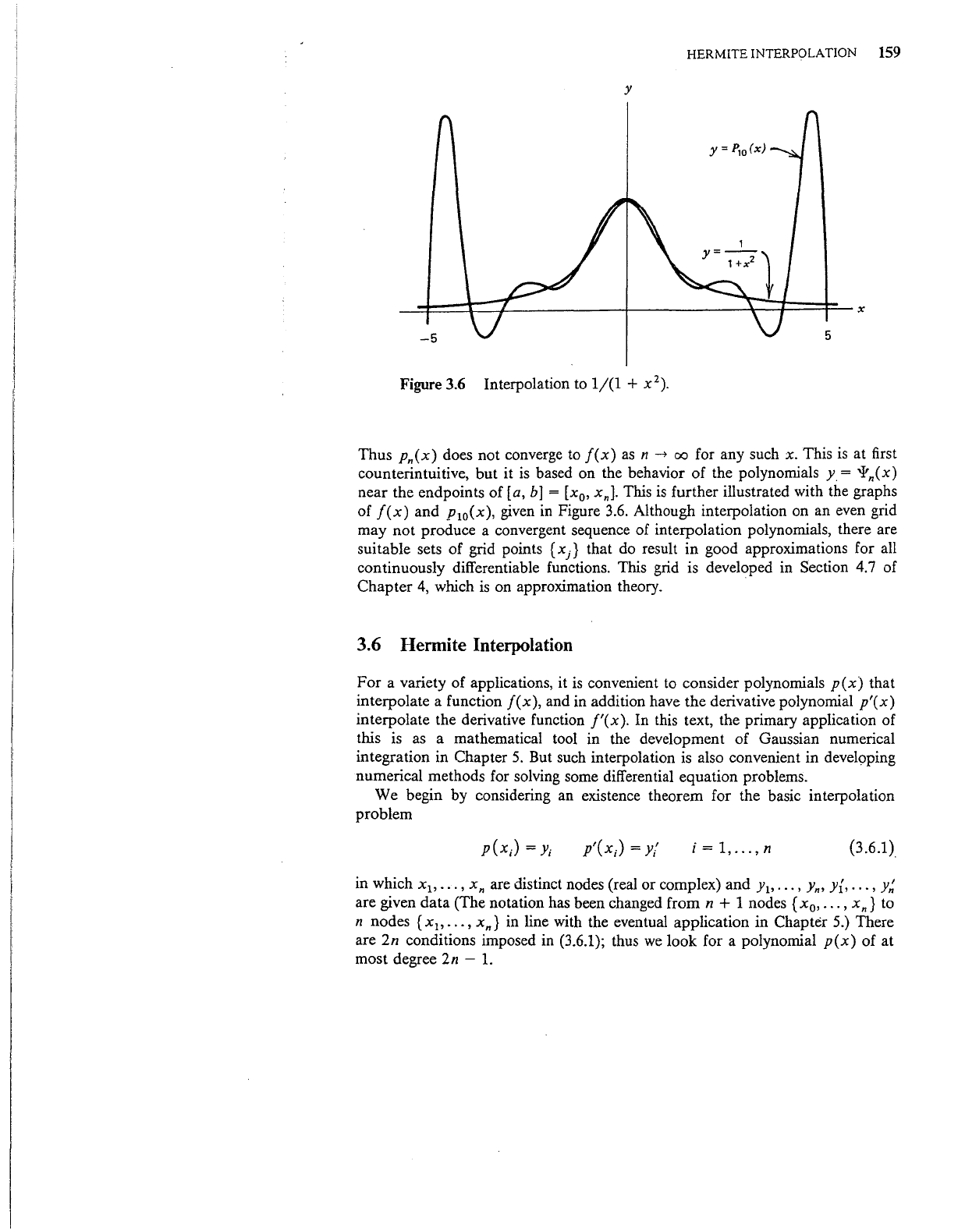
Figure
3.6
Interpolation to
1/(1
+ x
2
).
Thus Pn(x) does not converge to
f(x)
as
n ~
oo
for any such x. This
is
at first
counterintuitive, but it
is
based on the behavior of the polynomials y = 'l'n(x)
near the endpoints of
[a,
b]
= [x
0
,
xn].
This
is
further illustrated with the graphs
of
f(x)
and p
10
(x),
given
in
Figure 3.6. Although interpolation on an even grid
may
not
produce a convergent sequence of interpolation polynomials, there are
suitable sets of grid points {
xj}
that do result in good approximations for all
continuously differentiable functions. This grid is developed in Section 4.7 of
Chapter
4,
which
is
on approximation theory. ·
3.6 Hermite Interpolation
For a variety of applications, it
is
convenient
to
consider polynomials
p(x)
that
interpolate a function
f(x),
and in addition have the derivative polynomial
p'(x)
interpolate the derivative function
f'(x).
In this text, the primary application of
this
is
as a mathematical tool in the development of Gaussian numerical
integration in Chapter
5.
But such interpolation
is
also convenient in devel()ping
numerical methods for solving some differential equation problems.
We begin by considering an existence theorem for the basic interpolation
problem
p(x;)
=
Y;
p'(x;)
= y(
i = 1,
...
, n (3.6.1)
in which x
1
,
...
, xn are distinct nodes (real or complex) and
Yl·
...
,
Yn•
y{,
...
,
y;
are given
data
(The notation has been changed from n + 1 nodes { x
0
,
•••
, xn} to
n nodes { x
1
,
•••
, xn}
in
line with the eventual application in Chapter
5.)
There
are
2n
conditions imposed
in
(3.6.1); thus
we
look for a polynomial
p(x)
of at
most degree
2n -
1.
160 INTERPOLATION THEORY
To
deal with the existence and uniqueness for
p(x),
we
generalize the third
proof
of Theorem
3.1.
In
line with previous notation in Section 3.1, let
i',.(x)
=
(x-
x
1
)
• • •
(x-
x,.)
/.(x)
=
(x-
x
1
) · · ·
(x-
X;_
1
)(x-
X;+
1
)
· · ·
(x-
x,.)
1
(x.-
X ) • • •
(x.-
X·
)(x.-
X·
)
''
•
(x-
X )
1 1 r
r-1
1
1+1
n
h;(x)
=
(x-
x;)[l;(x)]
2
h;(x)
=
[1-
2/f(x;)(x-
x;)] [l;(x)]
2
Then
for i, j = 1,
...
, n,
hj(x)
=
h;(x)
= 0
1
~
i,
j
~
n
i=Fj
i=j
The
interpolating polynomial for (3.6.1)
is
given by
n n
H,.(x) = L Y;h;(x) + L y;'h;(x)
i=1
i=l
(3.6.2)
(3.6.3)
(3.6.4)
To
show the uniqueness
of
H,.(x), suppose there is a second polynomial
G(x)
that
satisfies (3.6.1) with degree
~
2n
-
1.
DefineR
= H -
G.
Then from (3.6.1)
R(x;)
= R'(x;) = 0
i=1,2,
...
,n
where R is a polynomial
of
degree~
2n
- 1, with n double roots, x
1
,
x
2
,
•.•
, x,..
This
can
be
true only if
for some polynomial
q(x).
If
q(x)
'¢
0,
then degree
R(x)
~
2n, a contradiction.
Therefore we
must
have
R(x)
= 0.
To
obtain
a more computable form than (3.6.4)
and
an error term, first
consider the polynomial interpolating
/(x)
at
nodes z
1
, z
2
,
...
, z
2
,.,
written in the
Newton
divided difference form:
P2n-1(x) =
/(z1)
+
(x-
zr)/[zl,
z2]
+
...
+
(x-
z
1
) · · ·
(x-
z
2
,._
1
)/[z
1
,
...
, z
2
,.]
(3.6.5)
For
the error,
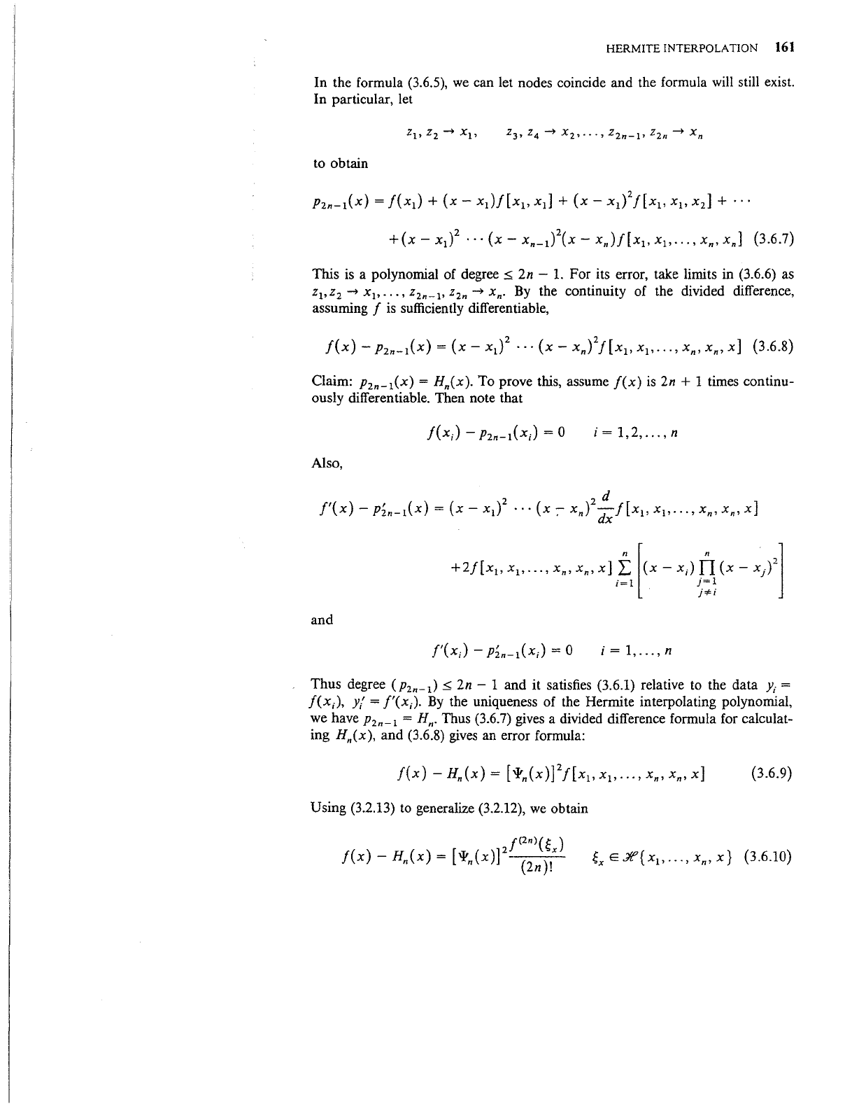
HERMITE INTERPOLATION
161
In the formula (3.6.5),
we
can let nodes coincide and the formula
will
still exist.
In particular, let
to obtain
This
is
a polynomial of degree
.:S
2n -
1.
For its error, take limits in (3.6.6) as
z
1
,z
2
~ x
1
,
•••
, z
2
n-l• z
2
n
~
xn.
By
the continuity of the divided difference,
assuming
f
is
sufficiently differentiable,
Claim:
P2n-
1
(x)
= Hn(x). To prove this, assume
f(x)
is
2n + 1 times continu-
ously differentiable. Then note that
f(x;)-
P2n-l(x;)
= 0
i =
1,2,
...
, n
Also,
+2/[xl,
X
1
,
...
,
xn,
xn,
x]
f
[(x-
x;)
TI
(x-
xj)
2
]
i=l
j=l
j*i
and
i
=I,
...
, n
Thus degree
(p
2
n_
1
)
.:S
2n-
1 and it satisfies (3.6.1) relative to the data
Y;
=
f(x;),
Y/
=
f'(x;).
By
the uniqueness of the Hermite interpolating polynomial,
we have
hn-l
=
Hn.
Thus (3.6.7) gives a divided difference formula for calculat-
ing
Hn(x),
and (3.6.8)
gives
an error formula:
(3.6.9)
Using (3.2.13) to generalize (3.2.12),
we
obtain
~xE£{x
1
,
...
,xn,x}
(3.6.10)
162 INTERPOLATION THEORY
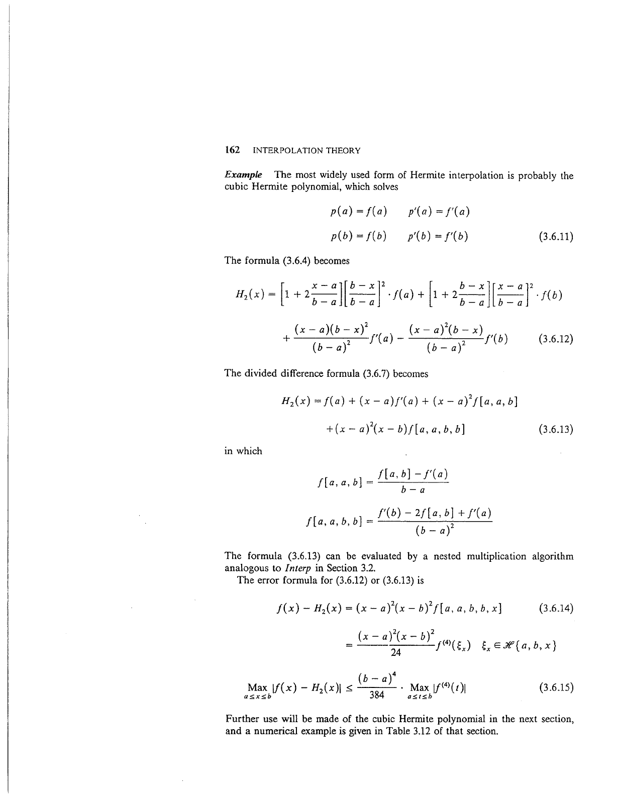
Example The most widely used form of Hermite interpolation
is
probably the
cubic Hermite polynomial, which solves
p(a)
=/(a)
p(b)=J(b)
The formula (3.6.4) becomes
p'(a)=f'(a)
p'(b) = J'(b)
(3.6.11)
[
x-a][b-x]2
[
b-x][x-a]z
H
2
(x) = 1 +
2--
--
·
f(a)
+ 1 +
2--
--
·
f(b)
b-a b-a
b-a
b-a
(x-
a)(b-
x)
2
(x-
a)
2
(b-
x)
+
(b-a)2
f'(a)-
(b-a)z
f'(b)
The divided difference formula (3.6.7) becomes
in which
H
2
(x)
=/(a)+
(x-
a)f'(a)
+
(x-
a)
2
f[a,
a,
b]
+(x-
a)
2
(x-
b)f[a,
a,
b,
b]
f[a,
b]-
f'(a)
f[a,
a,
b]
= b
_a
/'(b)-
2f[a,
b]
+
f'(a)
f[a,a,b,b]=
2
(b-
a)
(3.6.12)
(3.6.13)
The formula (3.6.13) can be evaluated
by
a nested multiplication algorithm
analogous to
Interp in Section
3.2.
The error formula
for
(3.6.12) or (3.6.13)
is
(3.6.14)
(x-a)~~x-b)2J<4>(gx)
gxE.n"{a,b,x}
(b-
a)
4
a~;:blf(x)-
H2(x)l
~
384
Max
l/<
4
>(t)l
a5,t5,b
(3.6.15)
Further use will be made of the cubic Hermite polynomial in the next section,
and a numerical example
is
given in Table
3.12
of that section.
PIECEWISE POLYNOMIAL INTERPOLATION
163
The
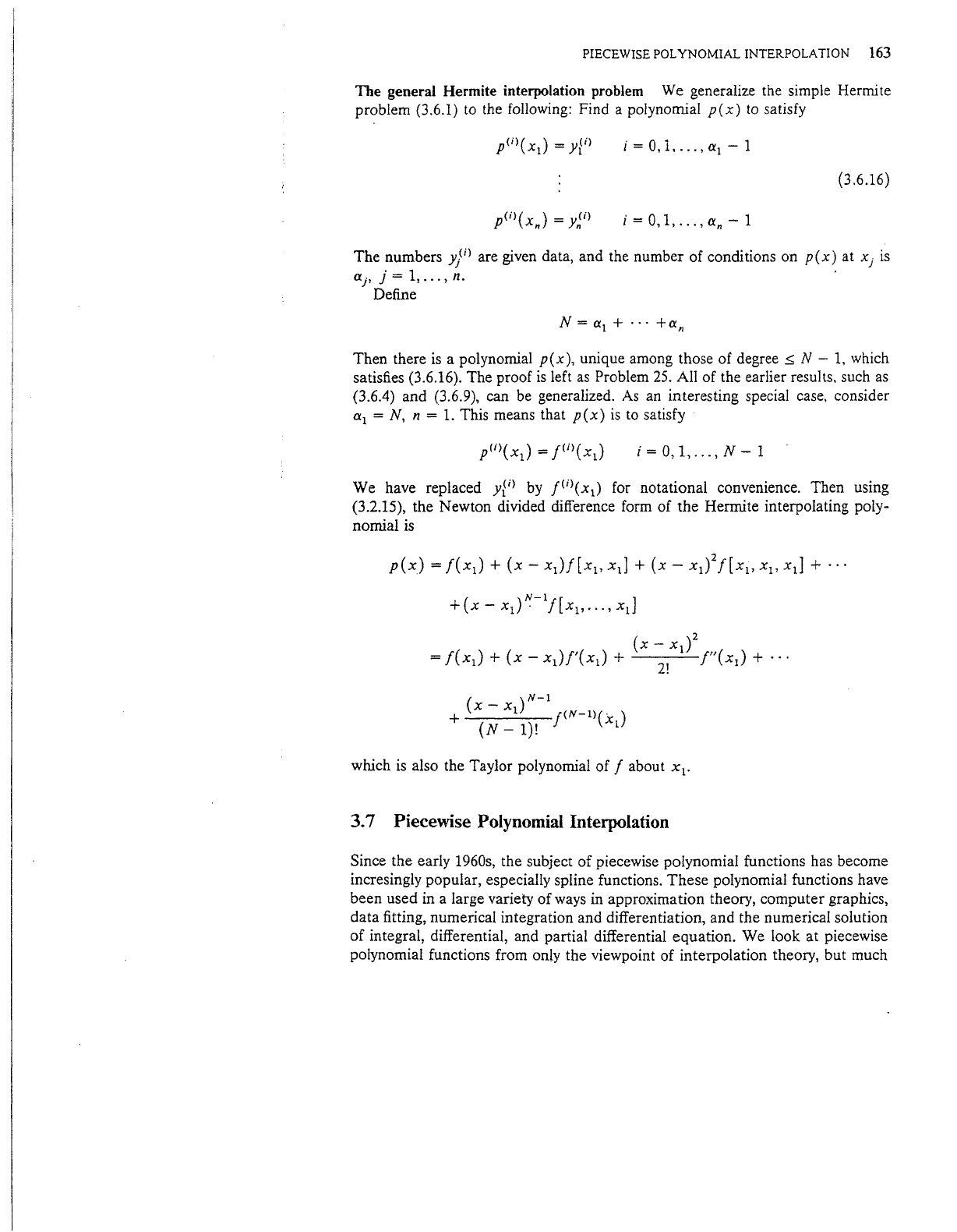
general Hermite interpolation problem We generalize the simple Hermite
problem (3.6.1) to the following: Find a polynomial
p(x)
to
satisfy
i=O,l,
...
,a
1
-1
(3.6.16)
i =
0,
1,
...
'
an
- 1
The
numbers
yji>
are given data, and the number of conditions on
p(x)
at x
1
is
a
1
,
j =
1,
...
, n. ·
Define
Then there
is
a polynomial
p(x),
unique among those of degree.::; N -
1,
which
satisfies (3.6.16). The proof
is
left
as
Problem
25.
All of the earlier results. such
as
(3.6.4) and (3.6.9), can be generalized.
As
an interesting special case, consider
a
1
= N, n =
1.
This means that
p(x)
is
to satisfy
i=O,l,
...
,N-1
We have replaced
yfil
by jU>(x
1
)
for notational convenience. Then using
(3.2.15), the Newton divided difference form of
the
Hermite interpolating poly-
nomial
is
p(x)
=
f(x
1
) +
(x-
x
1
)/[x
1
,
x
1
]
+
(x-
x
1
)
2
/[x
1
,
x
1
,
x
1
]
+ · · ·
+(x-
x
1
)N-
1
/(x
1
,
...
,
xJ
(x-
x )
2
=
f(x
1
) +
(x-
x
1
)f'(x
1
)
+
21
1
f"(x
1
)
+ · · ·
(
x-x)N-1
+
1
J<N-1>(x
)
(N-1)!
1
which
is
also the Taylor polynomial
off
about x
1
.
3. 7 Piecewise Polynomial Interpolation
Since the early 1960s, the subject
of
piecewise polynomial functions has become
incresingly popular, especially spline functions.
These
polynomial functions have
been used in a large variety
of
ways in approximation theory,
computer
graphics,
data fitting, numerical integration and differentiation, and the numerical solution
of
integral, differential, and partial differential equation.
We
look at piecewise
polynomial functions from only the viewpoint of interpolation theory, but much
164
INTERPOLATION THEORY
of
their
useful application occurs in some
other
area, with interpolation occurring
only
in
a peripheral way.
For
a piecewise polynomial function
p(x),
there is
an
associated grid:
-00
<
Xo
< X1 < · · · <
Xn
<
00
(3.7.1)
The
points
x
1
are
sometimes called knots, breakpoints,
or
nodes.
The
function
p(x)
is a polynomial on each
of
the subintervals
(3.7.2)
although
often
the
intervals
(-
oo,
x
0
]
and
[xn,
oo)
are
not
included. We-say
p(x)
is a piecewise polynomial
of
order r if the degree
of
p(x)
is less
than
ron
each
of
the
subintervals
in
(3.7.2).
No
restrictions
of
continuity need
be
placed
on
p(x)
or
its derivatives, although usually
p(x)
is continuous. In this section, we mostly
restrict ourselves to piecewise cubic polynomial functions (of
order
four). This
is
the
most
common
case in applications,
and
it simplifies the presentation
to
be
definite as
to
order.
One
way
of
classifying piecewise polynomial interpolation problems is as local
or
global.
For
the
local type
of
problem, the polynomial
p(x)
on
each subinterval
[x;_
1
,
x;] is completely determined
by
the interpolation
data
at
node
points
inside
and
neighboring [x;_
1
,
xJ
But for a global problem, the choice
of
p(x)
on
each
[x;-u
x;] is dependent
on
all of the interpolation data.
The
global problems
are
somewhat
more
complicated to study; the best known examples are the spline
functions,
to
be
defined later.
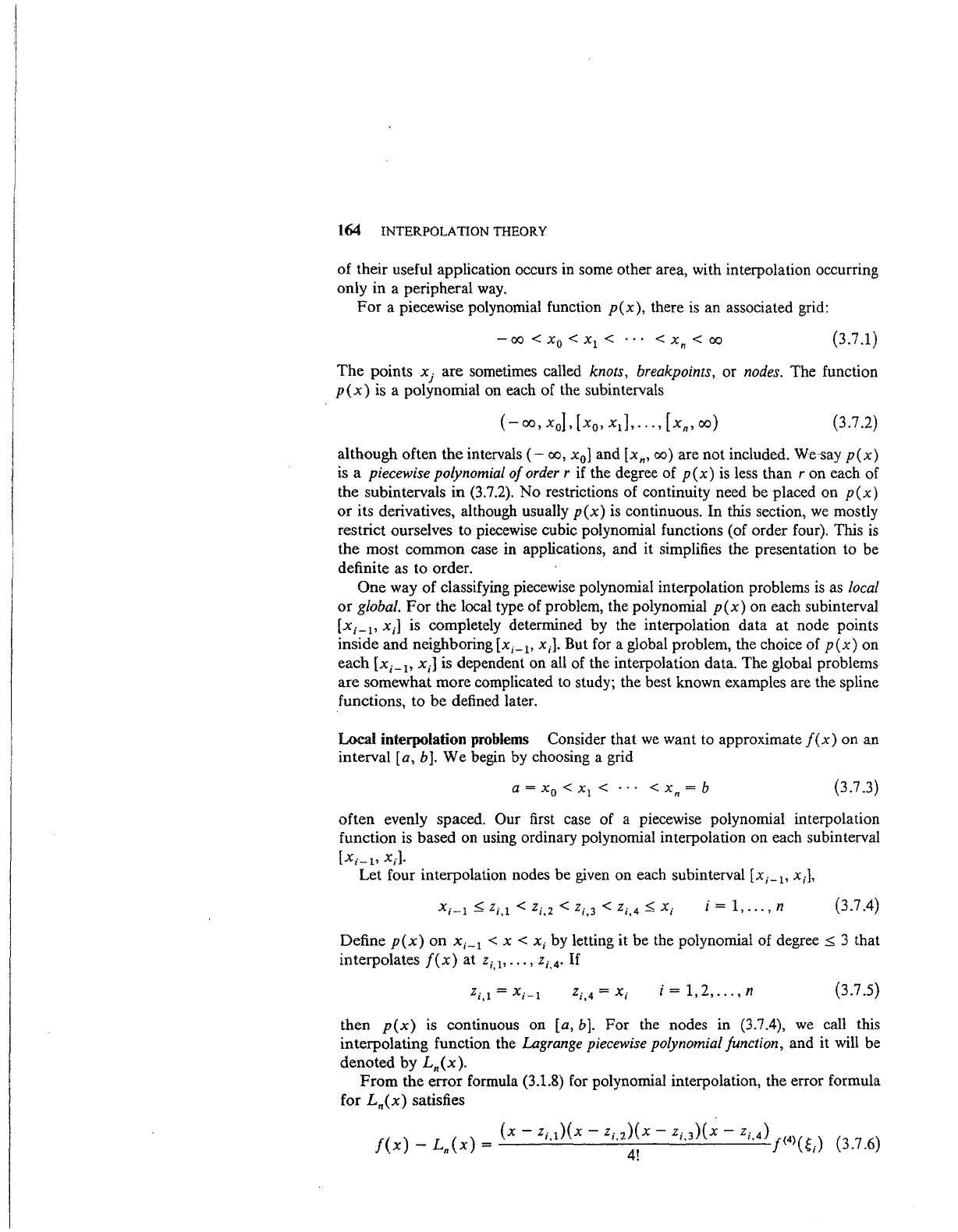
Local interpolation
problems
Consider that we
want
to approximate
f(x)
on
an
interval
[a, b
].
We
begin by choosing a grid
a =
Xo
< X
1
< · · · < X n = b
(3.7.3)
often
evenly spaced.
Our
first case
of
a piecewise polynomial interpolation
function
is
based
on using ordinary polynomial interpolation
on
each subinterval
[x;-1•
X;].
Let
four interpolation nodes
be
given
on
each subinterval [x;_
1
,
X;].
X;-!,::;;
Z;,!
<
Z;,2
<
Z;,J
<
Z;,
4
::::;
X;
i=1,
...
,n
(3.7 .4)
Define
p(x)
on
X;_
1
< x
<X;
by letting
it
be
the polynomial
of
degree::::; 3 that
interpolates
f(x)
at
z;,
1
,
...
,
z;,
4
•
If
Z;,!
=X;-!
Z;,
4
=X;
i =
1,2,
...
, n
(3.7 .5)
then
p(x)
is continuous
on
[a,
b].
For
the nodes
in
(3.7.4), we call this
interpolating
function the Lagrange piecewise polynomial function,
and
it
will be
denoted
by
Ln(x).
From
the
error
formula (3.1.8) for polynomial interpolation, the
error
formula
for
Ln(x)
satisfies
f(x)-
Ln(x)
=
(x-
Z;,l)(x-
Z;,z~~x-
z;,3)(x-
z;,4)
j<4l(~;)
(3.7.6)
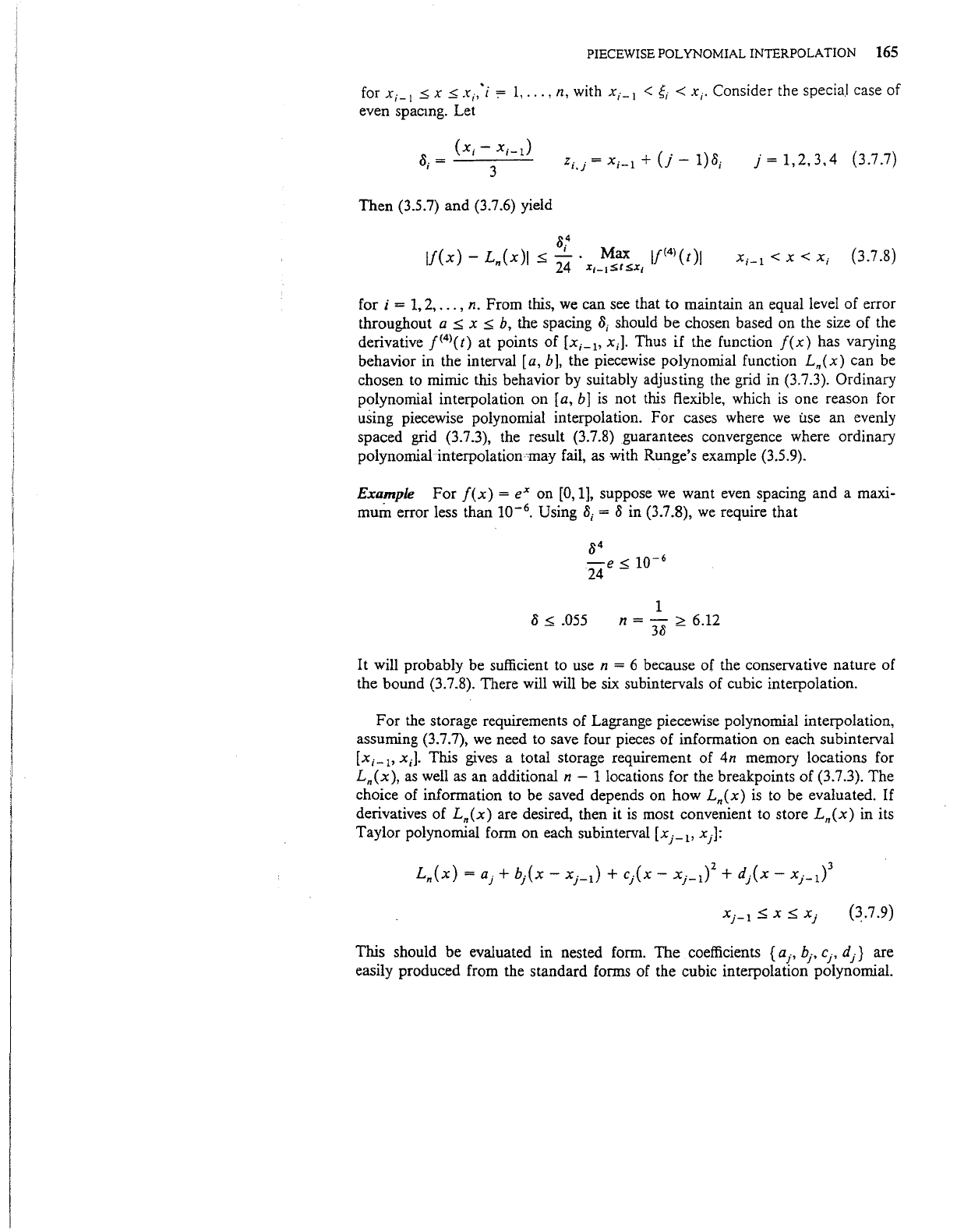
PIECEWISE POLYNOMIAL INTERPOLATION 165
for
X;_
1
s x s
x;:
i
:=
1,
...
,
n,
with
X;_
1
<
~;
<X;.
Consider the specia.l case of
even spacmg. Let
(x;-
X;_
1
)
8.=----
, 3
Z;,j
=
X;-1
+
(j-
1)o;
j =
1,2,3,4
(3.7.7)
Then (3.5.7) and (3.7.6) yield
X;-1
<X<
X;
(3.7.8)
for i =
1,
2,
...
, n. From this,
we
can
see
that to maintain an equal level of error
throughout a
s x s b, the spacing
8;
should be chosen based on the size of the
derivative
J<
4
>(t) at points of [x;_
1
,
x;). Thus
if
the function
f(x)
has varying
behavior
in
the interval
[a,
bJ,
the piecewise polynomial function
Ln(x)
can be
chosen to mimic this behavior by suitably adjusting the grid in
(3.7.3). Ordinary
polynomial interpolation on
[a,
b]
is
not
this
flexible, which
is
one reason for
using piecewise polynomial interpolation. For cases where
we
use an evenly
spaced grid
(3.7.3), the result (3.7.8) guarantees convergence where ordinary
polynomiahnterpolation-may
fail,
as with Runge's example (3.5.9).
Example For
f(x)
=ex
on
[0,
1],
suppose
we
want even spacing and a maxi-
mum error less than
10-
6
•
Using
8;
= o in (3.7.8),
we
require that
04
-e
<
10-
6
24 -
0 s .055
1
n
=-
>
612
3o
- ·
It will probably be sufficient to use n = 6 because of the conservative nature of
the bound
(3.7.8). There will will be six subintervals of cubic interpolation.
For the storage requirements of Lagrange piecewise polynomial interpolation,
assuming
(3.7.7),
we
need to save four pieces of information on each subinterval
[x;_
1
,
x;). This
gives
a total storage requirement of 4n memory locations for
Ln(x),
as
well
as an additional
n-
1locations for the breakpoints of (3.7.3). The
choice of information to be saved depends on how
Ln(x)
is
to
be evaluated.
If
derivatives of
Ln(x)
are desired, then it
is
most convenient to store
Ln(x)
in its
Taylor polynomial form on each subinterval
[x
1
_
1
,
x
1
]:
(~.7.9)
This should be evaluated in nested form. The coefficients { a
1
,
b
1
,
c
1
,
d
1
}
are
easily produced from the standard forms of the cubic interpolation polynomial.
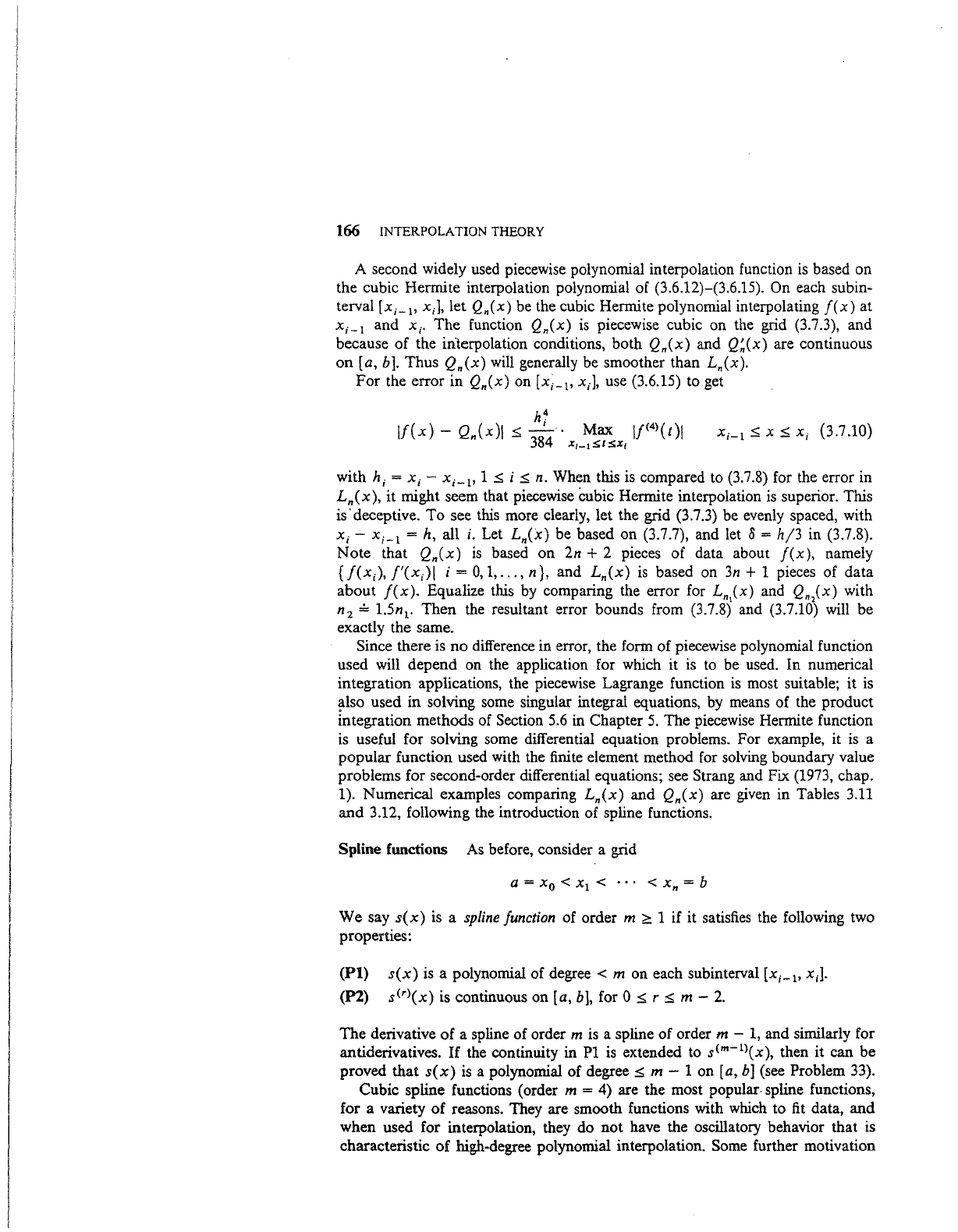
166 INTERPOLATION THEORY
A second widely used piecewise polynomial interpolation function
is
based on
the cubic Hermite interpolation polynomial of
(3.6.12)-(3.6.15). On each subin-
terval
[x;_
1
,
X;),
let Qn(x) be the cubic Hermite polynomial interpolating
f(x)
at
X;_
1
and
X;.
The
function
Qn(x)
is
piecewise cubic on the grid (3.7.3), and
because of the interpolation conditions, both
Q"(x)
and
Q~(x)
are continuous
on
[a,
bJ.
Thus
Qn(x)
will
generally be smoother than
L.(x).
For
the error in Qn(x) on [x;_
1
,
X;),
use (3.6.15) to get
X;-1
.$;X.$;
X;
(3.7 .10)
with h;
=X;-
X;_
1
,
1
.s;
i
.s;
n. When this is compared to (3.7.8) for the error in
Ln(x),
it
might seem that piecewise cubic Hermite interpolation
is
superior. This
is· deceptive.
To
see this more clearly, let the grid (3.7.3) be evenly spaced, with
X;-
x;_
1
= h, all
i.
Let Ln(x) be based on (3.7.7), and let o =
h/3
in (3.7.8).
Note
that
Qn(x)
is
based on 2n + 2 pieces of data about
f(x),
namely
{f(x;),f'(x;)i
i = 0,1,
...
,n},
and
Ln(x)
is
based on
3n
+ 1 pieces of data
about
f(x).
Equalize this
by
comparing the error for
LnJx)
and Q"
2
(x)
with
n
2
= 1.5n
1
•
Then the resultant error bounds from (3.7.8) and (3.7.10) will be
exactly the same.
Since there is
no
difference in error, the form of piecewise polynomial function
used will depend on the application for which it
is
to
be used.
In
numerical
integration applications, the piecewise Lagrange function
is
most suitable; it
is
!J.lso
used in solving some singular integral equations, by means of the product
integration methods of Section
5.6
in Chapter
5.
The piecewise Hermite function
is useful for solving some differential equation problems. For example, it is a
popular function used with the finite element method for solving boundary value
problems for second-order differential equations; see Strang and Fix
(1973, chap.
1). Numerical examples comparing
Ln(x)
and
Qn(x)
are given in Tables
3.11
and
3.12, following the introduction of spline functions.
Spline functions
As
before, consider a grid
a =
Xo
< X
1
< · • · <
Xn
= b
We say
s(x)
is a spline function of order m
2!
1 if it satisfies the following two
properties:
(Pl)
s(x)
is a polynomial of
degree<
m on each subinterval [x;_
1
,
x;].
(P2)
s<'>(x)
is continuous on [a,
bJ,
for 0
.s;
r
.s;
m-
2.
The
derivative
of
a spline of order m
is
a spline of order m -
1,
and similarly for
antiderivatives.
If
the continuity in
Pl
is
extended to
s<m-
1
>(x),
then
it
can be
proved that
s(x)
is
a polynomial of degree
.s;
m - 1 on
[a,
bJ
(see Problem 33).
Cubic spline functions (order
m = 4) are the most popular. spline functions,
for a variety
of
reasons. They are smooth functions with which to
fit
data,
and
when used for interpolation, they do not have the oscillatory behavior that is
characteristic
of
high-degree polynomial interpolation. Some further motivation
