Amano R.S., Sunden B. (Eds.) Computational Fluid Dynamics and Heat Transfer: Emerging Topics

Подождите немного. Документ загружается.

Sunden CH009.tex 25/8/2010 10: 57 Page 346

346 Computational Fluid Dynamics and Heat Transfer

(a)

a [W/(m

K )]a [W/(m

K )]

100

150

200

250

300

350

400

0 100 200 300 400 500 600 700

x(mm)

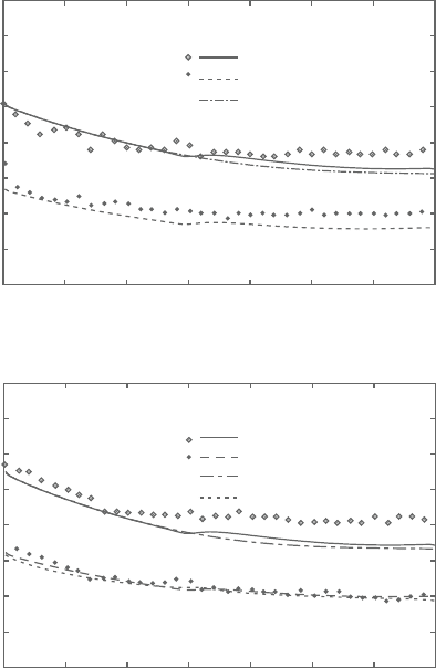
Element height = 0.5 mm: h = 0.55 mm

Expt. AWF + CLS

= 40 m/s

= 22 m/s

= 40 m/s; straight

(b)

100

150

200

250

300

350

400

0 100 200 300 400 500 600 700

x(mm)

Element height = 0.75 mm: h = 0.825 mm

Expt. AWF + CLS

= 40 m/s

= 22 m/s

= 40 m/s; straight

= 22 m/s; fine mesh

Figure 9.11. Heat transfer coefﬁcient distribution in convex rough wall boundary

layers at Pr=0.71.

Computations are consistent with this experimental observation. Note that the

present curvature effects are of the entrance region of the convex wall. Due to

the sudden change of the curvature rate, the pressure gradient becomes locally

strongernearthestartingpoint oftheconvexwallresultinginﬂowaccelerationand

thus heat transfer enhancement.

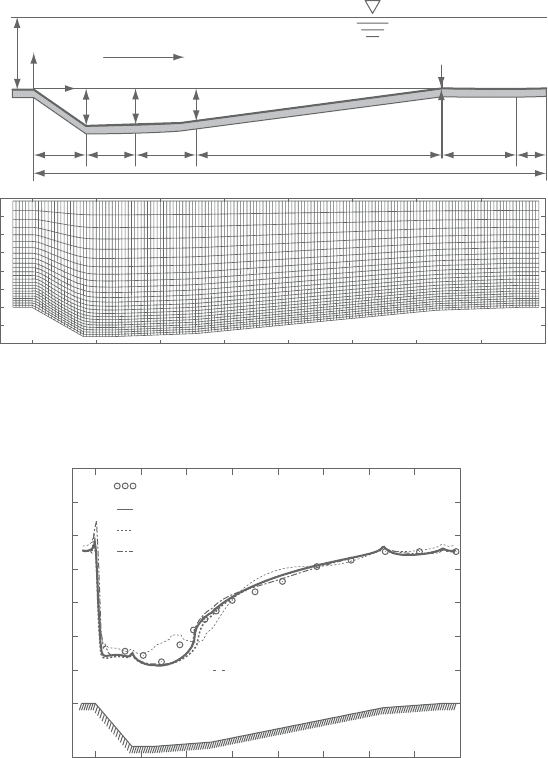
Sand dune ﬂow. Figure 9.12 shows the geometry and a computational mesh used

for a water ﬂow over a sand dune of van Mierlo and de Ruiter [29]. Their exper-

imental rig consisted of a row of 33 identical 2D sand dunes covered with sand

paper, whose averaged sand grain height was 2.5mm. Since they measured the

ﬂowﬁeld aroundoneofthe centraldunesofthe row, streamwiseperiodicboundary

conditions are imposed in the computation. In the experiments, the free surface

Sunden CH009.tex 25/8/2010 10: 57 Page 347

AWFs of turbulence for complex surface ﬂow phenomena 347

−0.1

−0.05

0.05

0.1

0.15

0.2

0.25

0.3

0 0.2 0.4 0.6 0.8 1 1.2 1.4 1.6

y (m)

x (m)

165 × 25

Water flow

160 100 250 750

1600

260 80

292

Figure 9.12. Dune proﬁle and computational g rid.

−0.05

0.0

0.05

0.1

0 0.2 0.4 0.6 0.8 1 1.2 1.4 1.6

x (m)

Expt.

Grid 165 × 25 (LWF + CLS)

Grid 329 × 50 (AWF + CLS)

Grid 165 × 50 (AWF + CLS)

Grid 165 × 25 (AWF + CLS)

Figure 9.13. Friction velocity over the sand dune.

was located at y =292mm and the bulk mean velocity was U

=0.633m/s. Thus,

the Reynolds numberbased on U

and thesurface heightwas 175,000.In this ﬂow,

a large recirculation zone appears behind the dune. Due to the ﬂow geometry, the

separation point is ﬁxed at x =0m as in a back-step ﬂow.

Figure 9.13 compares the predicted friction velocity distribution on meshes of

330×50, 165×50 and 165×25. In the ﬁnest and coarsest meshes, the heights of

the ﬁrst cell facing the wall are, respectively, 4 and 8mm, and larger than thegrain

height of 2.5mm which corresponds to h

75 at the inlet.The turbulence model

Sunden CH009.tex 25/8/2010 10: 57 Page 348

348 Computational Fluid Dynamics and Heat Transfer

applied is the cubic CLS k-ε model with the differential length-scale correction

term for the dissipation rate equation [30]. The lines of the predicted proﬁles are

almost identical to one another, proving that the AWF is rather insensitive to the

computational mesh. (In the following discussions on ﬂow ﬁeld quantities, results

by the ﬁnest mesh of 330×50 are used.)

Figure9.13 also showsthe result by theLWF.Although the LWF, equation (36)

should perform reasonably in ﬂat plate boundary layer type of ﬂows, it is obvious

that the LWF produces an unstable wiggled proﬁle in the recirculating region of

0m< x< 0.6m. The computational costs by the AWF and the LWF are almost

the same as each other, with the more complex algebraic expressions of theAWF

requiring slightly more processing time.

Figure 9.14 compares ﬂow ﬁeld quantities predicted by the CLS and the LS

models with the AWF. In the distribution of the mean velocity and the Reynolds

shear stress, both models agree reasonably well with the experiments as shown in

Figure 9.14a and b while the CLS model predicts the streamwise normal stress

better than the LS model (Figure 9.14c).These predictive trends of the models are

consistent with those in separating ﬂows by the original LRN versions and thus it

is conﬁrmed that coupling with the AWF preserves the original capabilities of the

LRN models.

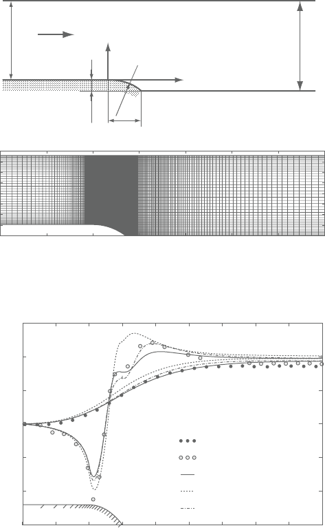
Ramp ﬂow. Figure 9.15 illustrates the ﬂow geometry and a typical computational

mesh (220×40) used for the computations of the channel ﬂows with a ramp on

the bottom wall by Song and Eaton [31]. A 2D wind tunnel whose height was

152mm with a ramp (height H =21mm, length L=70mm, radius R=127mm)

was used in their experiments. Air ﬂowed from the left at a free stream velocity

=20m/s with developed turbulence (Re

=3,400 at x =0mm for the smooth

wallcase; Re

=3,900 fortherough wall case). Since for the rough wall case sand

paper with an averaged grain height of 1.2mm, which corresponds to h

100 at

x =0mm, covered theramp part, the heightof theﬁrstcomputational cellfrom the

wall is set as 1.5mm. (Note that since the location of the separation point is not

ﬁxed in this ﬂow case, the grid sensitivity test, which is not shown here, suggests

that unlike in the other ﬂow cases large wall adjacent cell heights affect prediction

of the recirculation zone.) This ﬂow ﬁeld includes an adverse pressure gradient

along the wall and a recirculating ﬂow whose separation point is not ﬁxed, unlike

in the sand dune ﬂow. The measured velocity ﬁelds implied that the recirculation

regionextendedbetween0.74≤x



(:x/L)≤1.36and0.74< x



≤ 1.76inthesmooth

and rough wall cases, respectively. Thus, relatively ﬁner streamwise resolution is

applied to the computational mesh around the ramp part.

Figure 9.16 compares the predicted pressure coefﬁcients of the smooth wall

case by the AWF and the standard LWF with the results of the LRN computation.

The turbulence model used is the CLS model. The ﬁrst grid nodes from the wall

) are located at y

=15∼150 for the wall-function models while those for the

LRN are located at y

≤0.2. (The mesh used for the LRN case has 100 cells in

they direction.)Obviously, theAWFproducesproﬁlesthatareclosertothoseofthe

experiment than the proﬁles of the LWF model.TheAWF reasonably captures the

Sunden CH009.tex 25/8/2010 10: 57 Page 349

AWFs of turbulence for complex surface ﬂow phenomena 349

(c)

−0.1

−0.05

0.05

0.1

0.15

0.2

0.25

0.3

x (m)

0 0.2 0.4 0.6 0.8 1 1.2

0.0 0.3

1.4 1.6 1.8

Expt.

AWF+ CLS

AWF+LS

1.58x = 0.06 0.21 0.37 0.60 0.82 0.97 1.12 1.27 1.42

uu/U

(b)

−0.1

−0.05

0.05

0.1

0.15

0.2

0.25

0.3

x (m)

0 0.2 0.4 0.6 0.8 1 1.2 1.4 1.6 1.8

1.58x = 0.06 0.21 0.37 0.60 0.82 0.97 1.12 1.27 1.42

0.0 0.03

Expt.

AWF + CLS

AWF+LS

−uν/U

(a)

−0.1

−0.05

0.05

0.1

0.15

0.2

0.25

0.3

x (m)

y (m)y (m)y (m)

0 0.2 0.4 0.6 0.8 1 1.2 1.4 1.6 1.8

1.58x = 0.06 0.21 0.37 0.60 0.82 0.97 1.12 1.27 1.42

0.0 1.5

Expt.

AWF + CLS

AWF+LS

U/U

Figure 9.14. Mean velocityand Reynoldsstress distributionof thesanddune ﬂow.

effectsofadversepressuregradientsduetotheinclusionofthesensitivitytopressure

gradients in its form. Hence, its predictive tendency is similar to that of the LRN

model.

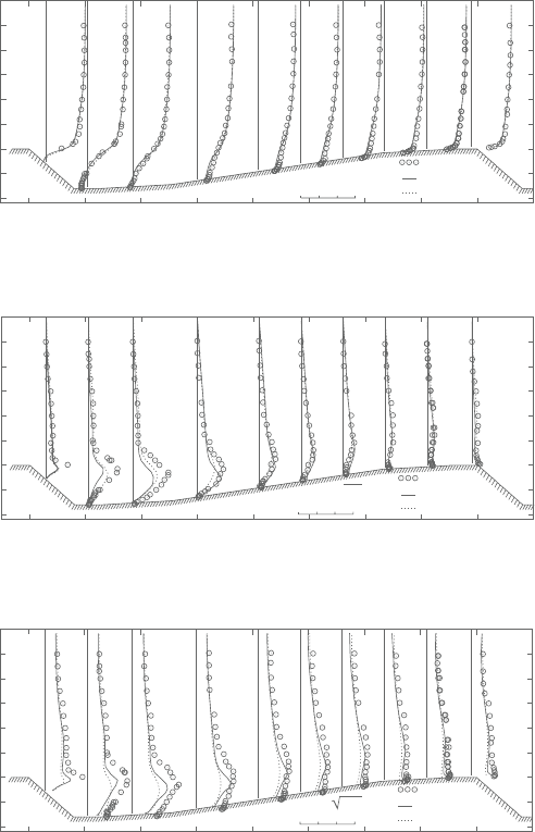
Figure 9.17a compares the mean velocity proﬁles for both the smooth and

rough wall cases. For both the cases, the agreement between the experiments

and the predictions by the AWF coupled to the CLS model is reasonably good.

Sunden CH009.tex 25/8/2010 10: 57 Page 350

350 Computational Fluid Dynamics and Heat Transfer

L (70)

R (127)

H (21)

152

131

Flow

100

120

140

160

−200 −100

0 100 200 300 400 500

y (mm)

x (mm)

220×40

Figure 9.15. Ramp geometry and computational grid.

−0.3

−0.2

−0.1

0.1

0.2

0.3

−2 −1

0 1 2 3 4 5 6 7

x ′

Top wall (smooth), Expt.

Bottom wall (smooth), Expt.

AWF y

= 15∼150

LWF y

= 15∼150

LRN y

= ∼0.2

Figure 9.16. Pressurecoefﬁcientdistributionofthesmoothrampﬂow;CLSisused

in all the computations.

The predicted recirculation zones are 0.69< x



< 1.40 and 0.57< x



< 1.60 in the

smooth and rough wall cases, respectively.They, however, do not correspond well

with the experimentally estimated ones. Figure 9.17b–d compare the distribution

of the Reynolds stresses at the corresponding locations to those in Figure 9.17a.

(The values are normalised by the reference friction velocity U

τ,ref

at x



=−2.0.)

Theagreementbetweenthepredictionandtheexperimentsisagainreasonablygood

for each quantity.

Sunden CH009.tex 25/8/2010 10: 57 Page 351

AWFs of turbulence for complex surface ﬂow phenomena 351

x’= –2.00 0.00 0.50 0.74 1.00 1.36 1.76 2.00 4.00 7.00

(b)

–1

–0.5

0.5

1.5

2.5

y/H

–uν/U

τ,ref

Expt.(rough)

Expt.(smooth)

AWF+CLS(rough)

AWF+CLS(smooth)

0.03.0

x’= –2.00 0.00 0.50 0.74 1.00 1.36 1.76 2.00 4.00 7.00

(c)

–1

–0.5

0.5

1.5

2.5

y/H

√

uu/U

τ,ref

Expt.(rough)

Expt.(smooth)

AWF+CLS(rough)

AWF+CLS(smooth)

0.03.0

x’= –2.00 0.00 0.50 0.74 1.00 1.36 1.76 2.00 4.00 7.00

(d)

–1

–0.5

0.5

1.5

2.5

y/H

√

νν/U

,ref

Expt.(rough)

Expt.(smooth)

AWF+CLS(rough)

AWF+CLS(smooth)

0.03.0

(a)

–1

–0.5

0.5

1.5

2.5

y/H

x’= –2.00 0.00 0.50 0.74 1.00 1.36 1.76 2.00 4.00 7.00

Expt.(rough)

Expt.(smooth)

AWF+CLS(rough)

AWF+CLS(smooth)

0.0 1.5

U/U

Figure 9.17. Mean velocity and Reynolds stress distribution of the ramp ﬂow.

Sunden CH009.tex 25/8/2010 10: 57 Page 352

352 Computational Fluid Dynamics and Heat Transfer

9.4.4 AWF for permeable walls

Flows over permeable walls can be seen in many industrially impor tant devices

such as catalytic converters, metal foam heat exchangers and separators of fuel

cells. Some geophysical ﬂuid ﬂows, i.e. water ﬂows over river beds etc., are often

concerned as ﬂows over permeable surfaces as well.

The effects of a porous medium on the ﬂow in the interface region between the

porous wall and clear ﬂuid (named ‘interface region’hereafter) have been focused

on by many researchers. Due to the severer complexity of the ﬂow phenomena,

however,experimentalturbulent ﬂowstudiesintheinterfaceregionsareratherlim-

ited. Zippe and Graf [32] and others experimentally found that the friction factors

of turbulent ﬂows over permeable beds became higher than those over imperme-

able walls with the same surface roughness. The recent DNS study of the interface

regionbyBreugemetal. [33]alsoindicatedthatthefrictionvelocitybecamehigher

associated with the increase of the permeability. All these results imply that the

wallpermeabilityeffectsonturbulenceshouldbesolelytakeninto accountforﬂow

simulations.

This part, thus, introduces an attempt [11] to construct anAWF which includes

the effects ofthewallpermeability aswellas the wall roughness forcomputing the

interface regions over porous media.

Modelling for porous/ﬂuid interfacial turbulence

It is natural to consider a slip tangential velocity U

at the interface between a

clear ﬂuid ﬂow and a porous surface when one introduces a volume averaging

concept. Before discussing the slip velocity, it is essential to deﬁne a nominal

location of the interface. In some porous media, their outermost perimeter may

be reasonable as the interface [34]. This means when the pores are ﬁlled with

solidmaterial, asmoothimpermeableboundaryis recovered.However, incase that

a porous medium is composed of beads, the recovered impermeable surface has

some roughness by deﬁning the pores as the spaces surrounded by the beads.This

deﬁnition is consistent with those in the experiments by Zippe and Graf [32] and

y = 0

(b)(a)

Porous

medium

Figure 9.18. (a)Velocity proﬁle ofachannel ﬂow overa porous medium, (b)near-

wall cell.

Sunden CH009.tex 25/8/2010 10: 57 Page 353

AWFs of turbulence for complex surface ﬂow phenomena 353

others. Therefore, the surface roughness h of porous/ﬂuid interface is considered

as in Figure 9.18a and that the interface is located at the bottom of the roughness

elements. In order to obtain the tangential velocity U

at the interface (y =0), the

velocity distribution in a porous medium is estimated as follows.

Following Whitaker [35], the volume averaged Navier-Stokes equations for

incompressible ﬂows in isotropic porous media using the decomposition:

=u



+˜u

(47)

are:

∂u



∂t

+u



∂u



∂x

=−

∂p

∂x

+ ν

∂

u



∂x

−

∂τ

∂x

+ f

(48)

∂u



∂x

= 0 (49)

where p, ρ, ν, and ϕ are, respectively, the pressure, the density, the kinematic

viscosity of the ﬂuid and the porosityofthe porous medium.The volume averaged

values φ and φ

are superﬁcial and intrinsic averaged values of a variable φ,

respectively. (The superﬁcial averaging is deﬁned by taking average of a variable

over a volume element of the medium consisting of both solid and ﬂuid materials,

while the intrinsic averaging is deﬁned over a volume consisting of ﬂuid only.)

Between them the following relation exists:

φ=ϕφ

(50)

Although the sub-ﬁlter-scale dispersion ∂τ

/∂x

needs a closure model as in large

eddy simulations, it could be neglected in porous media since it is small enough

compared with the other ter ms. As in Whitaker [35], the drag force f

in isotropic

porous media can be parametrised as:

−ν

u



− ν

u



(51)

where K

and F

are, respectively, the permeability tensor and the Forchheimer

correction tensor. These tensors are empirically given by Macdonald et al. [37]

being based on the modiﬁed Ergun equation [36] as:

180(1 −ϕ)

@ AB C

(52)

100(1 −ϕ)

AB C



(u



)

(53)

where d

is the mean particle diameter.

Sunden CH009.tex 25/8/2010 10: 57 Page 354

354 Computational Fluid Dynamics and Heat Transfer

Thus, by the Reynolds averaging of the volume averaged momentum equa-

tions one can obtain the following equations for a developed turbulent ﬂow in a

homogeneous porous medium:

0 =−

∂P

∂x

−

∂

∂y

∂

∂y

−

U −

νϕF

qu

(54)

0 =−

∂P

∂y

−

∂

∂y

−

νϕF

qv

(55)

where q=

u



u



, u

= (u



− u



)(u



− u



), U =u, and

P =

p

In laminar ﬂow cases where the permeability Reynolds number Re

≡

√

/ν, which is based on the permeability K and the friction velocity U

,is

sufﬁciently small, the Reynolds stress and the Forchheimer drag terms can be

neglected:

0 =−

∂P

∂x

∂

∂y

−

U (56)

0 =−

∂P

∂y

(57)

The solutionof the above equations (56)and (57), namely,the Brinkman equations

[38] is a decaying exponential function which meets the interfacial (slip) velocity

at y =0 and the Darcy velocity U

deep inside the porous medium.

U = U

+ (U

− U

)exp





(58)

The Darcy velocity is:

=−

∂P

∂x

(59)

In the case of high Re

, turbulent diffusion and Forchheimer drag terms in the

momentumequationsshouldbeconsideredandthustheirgeneralanalyticalsolution

cannot be easily obtained. Breugem et al. [33] found that a good approximation

of the turbulent ﬂow inside the porous media can be obtained by the following

exponential formula:

U  U

+ (U

− U

)exp





(60)

where α

is an empirical coefﬁcient. If Re

is small enough, α

=1. In very large

cases, where the turbulent diffusion and the Forchheimer drag terms should

Sunden CH009.tex 25/8/2010 10: 57 Page 355

AWFs of turbulence for complex surface ﬂow phenomena 355

balance each other out:

−

∂

∂y



νϕF

qu

(61)

TheReynoldsstressestimatedwiththeeddyviscosity(ν

 u

y; u

isanappropriate

velocity scale) and the velocity gradient from equation (60) leads to

−

uv = ν

∂U

∂y

 u

 α

(62)

then the LHS of equation (61) may be rewritten as

−

∂

∂y

 α

(63)

Thus, α

can be estimated as



νϕF

⇒ α

 ν

F (64)

Therefore, the following form can be a model for α

= f

+ (1 −f

)ν

F (65)

= exp



−



(66)

bridgingbetween1andν

√

ϕ/KFdependingonthepermeability. Byreferringtothe

distributionof thecoefﬁcient α

obtainedfrom theDNS[33], themodel coefﬁcient

can be functionalised as

0.68

(67)

Hence

= exp



−

1.68



(68)

(Note thatthe aboveform isrewrittenin a different way for theAWF as inequation

(73).)

Consequently, the slip velocity U

can be expressed as

= U

∂U/∂y|

y=0

√

ϕ/K

(69)

with the velocity gradient ∂U/∂y|

y=0

given by the AWF.