Amano R.S., Sunden B. (Eds.) Computational Fluid Dynamics and Heat Transfer: Emerging Topics

Подождите немного. Документ загружается.

Sunden CH009.tex 25/8/2010 10: 57 Page 356

356 Computational Fluid Dynamics and Heat Transfer

In theAWF, the wall shear stress isobtainedby theanalytical solution ofa sim-

pliﬁed near-wall version of thetransport equationfor the wall-parallelmomentum.

Theresultantshearstressformhereisthesameasthatfortheroughwallturbulence

but with the slip velocity U

in the integration constant A

Since thewall permeability alsomakes the ﬂowmore turbulent, y

∗

should have

its dependency. Equation (38) is thus further modiﬁed as

∗

= y

∗



1 −(h

∗

/70)

− f



(70)

where f

is a function of the permeability. By referring to the experiments and

the DNS data [32, 33], the range of y

∗

which depends on the wall permeability

is estimated. Considering the roughness effects in y

∗

, the optimised function in

equation (70) for the permeability effects is

= 3.7



1 −exp

−



∗



>

(71)

whereK

∗

√

/ν. In thisform, K

∗

is usedrather thanRe

since theAWF uses

√

for the velocity scale. In order to keep consistency with such normalisation,

Equation (68) is rewritten as

 exp



−

∗1.68

250



(72)

using the relation of Re

 c

1/4

∗

. The following modiﬁed form, however, is

employed after further tuning of the model function

= exp



−

∗1.76

180



(73)

Examples of applications

Permeable-wallchannelﬂows. Inordertoconﬁrmtheperformanceofthemethod,

computationsoffullydevelopedturbulentﬂowsinaplanechannelwithapermeable

bottomwallaty/H =0andasolidtopwallaty/H =1(seeFigure9.18a)areshown

here. The considered ﬂow conditions are the same as those in the DNS [33]. The

mean diameter of the particle composing the permeable beds is d

/H =0.01 and

their porosity areϕ =0.95,0.80,0.60,0.00.The permeability and the Forchheimer

termarethenobtainedbyequations(52)and(53).ThebulkﬂowReynoldsnumberis

=5,500inallthecases.Theroughnessheightisconsideredtobeh=d

inthis

practice.Thegridcellnumberusedisonly10inthewallnormaldirectionduetothe

use of the wall-function approach for such relatively low Reynolds number ﬂows.

The turbulencemodels usedare the standardk-ε model[4] and thetwo-component

limit (TCL) second moment closure of Craft and Launder [39].

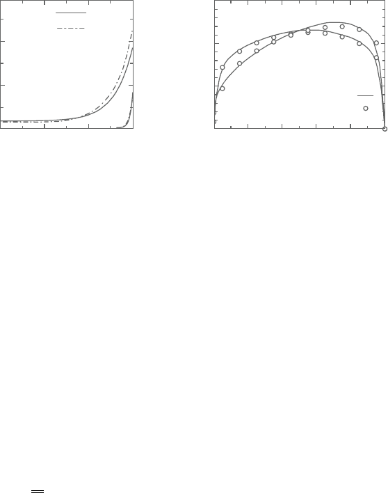
Figure 9.19a compares the mean velocity distribution inside the porous walls.

The obtained velocity proﬁles are from equation (60). Whilst there can be seen

Sunden CH009.tex 25/8/2010 10: 57 Page 357

AWFs of turbulence for complex surface ﬂow phenomena 357

0.3

1.5

1.0

0.5

0.95

w = 0.80

w = 0.95

0.0

0.80

Re = 5500

0.0 0.2 0.4 0.6 0.8 1.0

Present

DNS

0.2

0.1

0.0

y/H

(b)(a)

−0.15 −0.10 −0.05 0.00

U/U

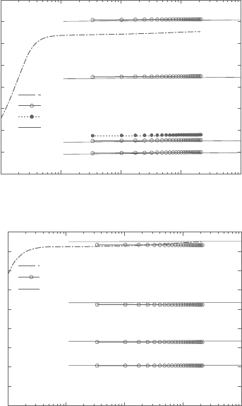
Figure 9.19. Meanvelocitydistribution:(a)insideporouswalls,(b)channelregion.

a margin to be improved in the comparison between the present and the DNS

results in the case of ϕ =0.95, the agreement is virtually perfect in the case of

ϕ =0.80.

The mean velocity distribution in the channel region is compared in Figure

9.19b. Itis obvious thatthe computationwell reproducesthe characteristicvelocity

proﬁles near the permeable walls.

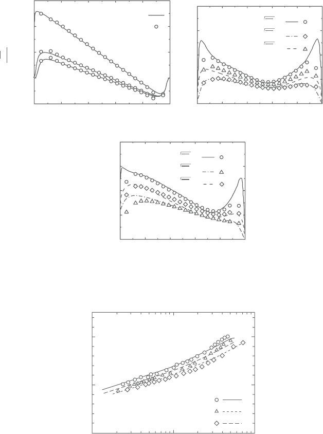
The AWF is also applicable to the second moment closures. Figure 9.20a–c

compares the obtained Reynolds stress distribution by the second moment closure

[39]. Due to the use of theAWF, it seems hard to capture the near wall peaks of the

Reynolds normal stresses as inFigure 9.20a and b. However, general tendencies of

the distribution proﬁles are satisfactorily reproduced by the present scheme.

Turbulent permeable boundary layer ﬂows. The other test cases are turbulent

boundary layerﬂowsover permeablewalls.Thesame ﬂow conditionsof the exper-

iments of Zippe and Graf [32] are imposed in the computations. The free stream

turbulenceis

= 0.35×10

−2

.TheReynoldsnumber basedon themomen-

tum thickness ranges Re

= 1.3−2.1 ×10

.Although it was not reported in Ref.

[32], the permeability can be estimated by equation (52) as K = 2.54 × 10

−9

since the experimentally used mean diameter of the ellipsoidal beads composing

thepermeablebed was d

= 2.883mm.The presently appliedporosity isϕ  0.30

considering the effects of non-spherical shapes of beads used in the experiments.

(The porosity of a fully packed body-centred cubic structure by spherical beads

is ϕ = 0.26. Zippe and Graf did not report about the porosity as well.) The grid

cell number used is 120 × 150 for the developing boundary layer computations.

The turbulence model used is the standard k-ε model of Launder and Spalding [4].

Since Zippe and Graf [32] also did not report the roughness height of their test

cases, it is presently estimated as h

 116 comparing the experimental velocity

proﬁle with the formula of Nikuradse [20]: Equation (36).

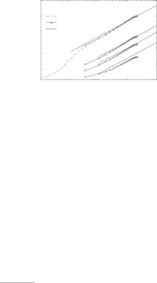
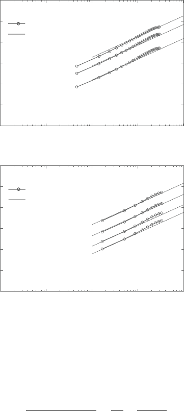
Figure 9.21 compares the mean velocity proﬁles where their boundary layer

thicknesses correspond to each other. The cases are R (non-permeable rough

Sunden CH009.tex 25/8/2010 10: 57 Page 358

358 Computational Fluid Dynamics and Heat Transfer

w = 0.95

w = 0.80

0.80

0.0

DNS :

DNS

present :

present

−1

0.0

(a) (b)

(c)

0.2 0.4 0.6 0.8 1.0

0.0

0.2 0.4 0.6 0.8 1.0

y/H

0.0

0.2 0.4 0.6 0.8 1.0

y/H

√

DNS

present

√

Figure 9.20. Reynolds stress distribution in permeable channel ﬂows.

Expt. present

100 1,000

10,000

12.5

P16.5

Figure 9.21. Mean velocity distribution in permeable boundary layers.

wall boundary layer), P

12.5

(permeable wall boundary layer with U

=12.5m/s)

and P

16.5

(permeable wall boundary layer with U

=16.5m/s). Obviously, the

presentschemereasonablyreproducestheexperimentallyobtainedvelocityproﬁles

with/without the permeability.

Sunden CH009.tex 25/8/2010 10: 57 Page 359

AWFs of turbulence for complex surface ﬂow phenomena 359

1 10 100 1,000 10,000

Re = 10

Pr = 0.71

0.2

0.1

0.025

LS(Pr = 0.71)

k-ε + AWF

Kader

Figure 9.22. MeantemperatureproﬁlesinturbulentsmoothchannelﬂowsatPr< 1.

9.4.5 AWF for high Prandtl number ﬂows

If oneconsiders to predict turbulentwall heattransfer of high Prandtlnumber ﬂuid

ﬂows such ascooling oil andICengine water-jacketﬂows, itis essential toanalyse

the thermal boundary layer which is much thinner than that of the ﬂow boundar y

layer. Thus, near-wall modelling which resolves the viscous sub-layer has been

thought to be essential for high Pr thermal ﬁelds. For example, at the development

ofanovelturbulentheatﬂuxmodelapplicabletogeneralPrcases,Rogersetal.[40]

supposed correct near-wall stress distribution and Suga andAbe [41] employed an

LRN nonlinear k-ε model. So and Sommer [42] also applied an LRN k-ε as well

as a near-wall stress transport model for ﬂows at Pr=1000.

However, even with the recent development of LRN heat transfer models,

wall-function approaches still attract industrial engineers. Its reasons are a high

computational cost of the LRN computation and difﬁculty of generating quality

near-wall grids for complex 3D ﬂow ﬁelds such as an IC engine water jacket.

AlthoughtheAWFperformsreasonablywellatPr< 1asshowninFigure9.22,

itsapplicabilitytohigherPrcaseshasnotbeendiscussedwellsofar.Therefore,this

part focuses on the improvement of the thermal AWF for high Pr turbulent ﬂows

with and without wall roughness [12].

High PrAWF for smooth wall heat transfer

IntheAWF forsmoothwallheattransfer,µ

variationisassumedthat µ

iszero for

∗

≤y

∗

=10.7and then increaseslinearlyas of equation(16). Since thetheoretical

Inthecases shown in Figure 9.22, theconstantPr

=0.9 is used forconvenience.However,

for lower Pr cases, it is well known that higher values of Pr

should be used [43]. There is

thus a tendency for the AWF to underpredict the mean temperature proﬁle, particularly, at

Pr=0.025.

Sunden CH009.tex 25/8/2010 10: 57 Page 360

360 Computational Fluid Dynamics and Heat Transfer

a′my

∗

/Pr

m/Pr :(air)

m/Pr : (oil)

/Pr

∗

Thermal diffusivities

am(y

∗

−y

∗

)/Pr

Figure 9.23. Near-wall thermal diffusivity distribution.

wall-limitingvariationof µ

is proportional toy

, this assumptiondoes not counta

certainamountofturbulentviscosityintheviscoussub-layer.Despitethat,itseffect

is not serious for ﬂow ﬁeld prediction since the contribution from the molecular

viscosity is more signiﬁcant in the sub-layer.This is also true for the ther mal ﬁeld

predictionofﬂuidswhosePrislessthan1.0. However, inhighPrﬂuidﬂowssuchas

oil ﬂows, since the effect of the molecular thermal diffusivity (µ/Pr)becomesvery

small as illustrated in Figure 9.23, it is then necessary to consider the contribution

from the turbulent thermal diffusivity inside the sub-layer. (Note that a prescribed

constant turbulent Prandtl number Pr

is assumed in Figure 9.23.)

In order to compensate the thermal diffusivity inside the sub-layer, Gerasimov

[17] introduced an ad hoc effective molecular Prandtl number as:

eff

1 +0.017Pr(1 + 2.9|F

− 1|)

1.5

(74)

where F

is a model function. This effective Pr approach was tailored for water

ﬂows.Thus, its performance in oil ﬂows whose Pr is over 100 is not guaranteed.

In order to improve the µ

proﬁle inside the sub-layer, it is assumed that the

proﬁleofEquation(16)isconnectedtoafunctionα



∗3

atthepointy

∗

,asillustrated

in Figure 9.23.

/µ =



∗3

, for 0 ≤ y

∗

≤ y

∗

α(y

∗

− y

∗

), for y

∗

≤ y

∗

(75)

Thus,



⎧

⎪

⎨

⎪

⎩

1 +



Pry

∗3

= 

θa

, for 0 ≤ y

∗

≤ y

∗

1 +

αPr(y

∗

− y

∗

)

= 

θb

, for y

∗

≤ y

∗

(76)

where µ

/Pr is the total thermal diffusivity. By referring to the near-wall proﬁle

of µ

in a DNS dataset, the value of y

∗

is optimised as y

∗

= 11.7 and thus α



Sunden CH009.tex 25/8/2010 10: 57 Page 361

AWFs of turbulence for complex surface ﬂow phenomena 361

obtainable as:



α(y

∗

− y

∗

)

∗3

(77)

Using equation (76), integration in equation (18) can be made. Although the

modiﬁcation of the modelis very simple, it makes the analytical integration a little

cumbersome as below.

When y

≤ y

, with P

=1/

θa

, P



= 1/

θb

, y

= 0,y

= y

and y

= y

the coefﬁcients D

and E

of equation (45) and (46) are:

= S

) −S

) +{S



) −S



)}

)



)

(78)

= S

) −S

) +S



) −S



)

(79)

+{S



) −S



)}

) −P



)



)

where P

= y

∗

, P



= y

∗



, S

∗

In the case of y

< y

, with y

= 0,y

= y

, they are:

= S

) −S

) (80)

= S

) −S

) (81)

(SeeAppendix B for the results of the integration of 1/

θa

etc.)

High PrAWF for rough wall heat transfer

Since theAWF heat transfermodel presented sofar was only validated in airﬂows,

the coefﬁcient C

needs recalibration inhigh Pr ﬂows and theobtained polynomial

form is:

= max(0,C

+ C

Pr +C

) (82)

=−0.48/h

∗

+ 0.0013, C

= 9.90/h

∗

− 0.0291

=−72.35/h

∗

+ 0.3067, C

= 98.98/h

∗

+ 0.2103

Since the rough wallAWF modiﬁes y

∗

of Equation (38) as:

∗

= y

∗

1 −



∗



= y

∗

− δ

(83)

the turbulent viscosity form of equation (75) changes to:

/µ =



∗

+ δ

)

, for y

∗

≤ y

∗

α(y

∗

− y

∗

), for y

∗

< y

∗

(84)

Sunden CH009.tex 25/8/2010 10: 57 Page 362

362 Computational Fluid Dynamics and Heat Transfer

Then, the thermal diffusivity has the following forms:



⎧

⎪

⎨

⎪

⎩

1 +



Pr(y

∗

+ δ

)

∞

+ C

max(0,1− y

∗

)

= 

θc

, for y

∗

< y

∗

1 +

αPr(y

∗

− y

∗

)

∞

+ C

max(0,1− y

∗

)

= 

θd

, for y

∗

≤ y

∗

(85)

The analytical solutions of energy equations then can be obtained in the four dif-

ferent cases illustrated in Figure 9.8. The resultant expressions for q

and A

are

of the same form as those presented so f ar. For cases (a) and (d) of Figure 9.8, D

and E

have theforms of Equations(78) and (79) withsome changes. For case (a),

they are P

= P



= 1/

θd

, y

= 0,y

= h and y

= y

. For case (d), they are

= P



= 1/

θc

, y

= 0,y

= h and y

= y

In cases (b) and (c), D

and E

have the following forms:

= S

) −S

) +{S



) −S



)}

)



)

+{S



)

(86)

− S



)}



)





)

= S

) −S

) +S



) −S



) +{S



) −S



)}

) −P



)



)

+ S



) −S



) +{S



) −S



)} (87)



) −P



)



)



)



)



) −P



)



)



For case (b), P

= 1/

θc

, P



= P



= 1/

θd

, y

= 0, y

= y

, y

= h, and

= y

. For case (c), P

= P



= 1/

θc

, P



= 1/

θd

, y

= 0,y

= h, y

= y

and y

= y

. (See Appendix B for the results of the integration of 1/

θc

etc.)

Examples of applications

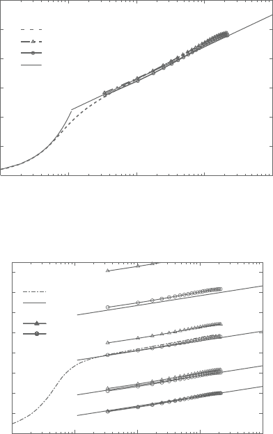
Smooth wall heat transfer. In order to conﬁrm the effects of the corrected turbu-

lentviscosityon theﬂow ﬁelds, Figure 9.24compares themean velocityproﬁles in

turbulentchannelﬂowsatthebulkReynoldsnumber, Re=10

. (Thestandardhigh

Reynolds number k-ε model [4] and the eddy diffusivity model with Pr

=0.9 are

used for the computation of the core ﬁelds of the present computations.)Although

theresultbytheµ

correctionalmostperfectlyliesonthelog-lawlineand therecan

be seen a slight discrepancy between the results with and without the correction,

both the results well accord with the LRN LS model and the log-law proﬁles. (The

meshes used for the AWF and the LRN computations have, respectively, 50 and

100 node points in the wall normal direction. Their ﬁrst cell heights are y

 30

and y

 0.2, respectively.) This conﬁrms that the correction in the momentum

equation may notbetotally necessary forengineeringﬂowﬁeld computations, and

thusthepresentschemedoesnot employthecorrectionfor theﬂowﬁeldAWF.This

Sunden CH009.tex 25/8/2010 10: 57 Page 363

AWFs of turbulence for complex surface ﬂow phenomena 363

1 10 100 1,000 10,000

Re = 10

k- + AWF(+corr.)

k- + AWF(no corr.)

Log − Law

Figure 9.24. Mean velocity proﬁles in turbulent smooth channel ﬂows.

}

Re = 10

Pr = 10.0

LS(Pr = 5.0)

Kader

k - ε+AWF(+ corr.)

k - ε+AWF(no corr.)

5.0

2.0

0.71

110

100 1,000 10,000

Figure 9.25. Mean temperature proﬁles in turbulent smooth channel ﬂows.

means that the correction of µ

is made only in the energy equation in the present

strategy.

Figure 9.25 clearly indicates that without the correction, the AWF does not

properlyreproducethelogarithmictemperatureproﬁlesinhighPrﬂowsofPr≥5.0.

Note that the experimentally suggested logarithmic distribution by Kader [44] for

a wide range of Pr is:

= 2.12ln(y

Pr) +(3.85Pr

1/3

− 1.3)

(88)

In the case of Pr=0.71, the proﬁles of the AWF with and without the correction

are virtually identical and conﬁrm that the near-wall correction of µ

is effective

for ﬂows at Pr> 1.0.

As shown in Figure 9.26a, the corrected AWF proves its good performance in

the range of 50≤Pr≤10

. However, both the LRN LS model and the AWF with

Sunden CH009.tex 25/8/2010 10: 57 Page 364

364 Computational Fluid Dynamics and Heat Transfer

(a)

200

400

600

800

1,000

1,200

1,400

1,600

1 10 100 1,000 10,000

500

100

LS (Pr = 500)

ε +AWF(Gerasimov,Pr = 500)

Kader

(b)

2,000

4,000

6,000

8,000

10,000

12,000

14,000

16,000

18,000

Re = 10

Pr = 10

Pr = 4 × 10

2 × 10

5 × 10

1 × 10

k-ε +AWF(+corr.)

LS (Pr = 2 × 10

)

Kader

ε +AWF(+corr.)

Figure 9.26. Mean temperature proﬁles in turbulent smooth channel ﬂows at

higher Pr.

Gerasimov’s [17] effective molecular Prandtl number scheme f ail to predict the

thermal ﬁeld at Pr=500. The former predicts the temperature too high and the

latter does too low. Figure 9.26b also conﬁrms that the corrected AWF performs

well up to Pr=4×10

though the LRN LS model predicts the thermal ﬁeld too

high. Note that the same grid resolution as that for Pr=5.0 is used in the LRN

computations. This reasonably implies that the grid resolution used is too coarse

andamuchﬁnergridisneededforsuchahighPrcomputationsbytheLRNmodels.

Obviously, it highlights the merit of using the AWF which does not require a ﬁner

grid resolution for a higher Pr ﬂow.

Rough wall heat transfer. Figure 9.27 compares the predicted temperature ﬁelds

of turbulent rough channel ﬂows of h/D=0.01 and 0.03, (D is channel height). In

thecasesofh/D =0.01,thecorrespondingroughnessReynoldsnumberish

 60

which is in the transitional roughness regime, while h/D = 0.03 corresponds

to h

 220 which is well in the fully rough regime. For each roughness case,

Sunden CH009.tex 25/8/2010 10: 57 Page 365

AWFs of turbulence for complex surface ﬂow phenomena 365

(a)

1 10 100 1,000 10,000

Pr = 10.0

5.0

0.71

Pr = 10.0

5.0

0.71

2.0

(b)

1 10 100 1,000 10,000

Re = 10

, h/D = 0.01

Re = 10

, h/D = 0.03

Kays-Crawford

k-ε+AWF(+corr.)

Kays-Crawford

k-ε + AWF(+corr.)

Figure 9.27. Mean temperature proﬁles in turbulent rough channel ﬂows.

it is obvious that the corrected AWF reasonably well reproduces the temperature

distribution for rough walls [45]:

0.8h

−0.2

−0.44

32.6y

(89)

where Pr

=0.9 and κ = 0.418. This correlation is based on the experiments of

Pr= 1.20 to 5.94 at the order of Re is 10

to 10

9.4.6 AWF for high Schmidt number ﬂows

Turbulentmasstransferacrossliquidinterfacesissometimesveryimportantinengi-

neering and environmental issues. For example, in order to estimate the amount of

the absorption of atmospheric CO

(carbon dioxide) at the sea surface, one should

consider predicting turbulent mass transfer across air–water interfaces. The difﬁ-

culty of analysing such a phenomenon comes from that the concentration (scalar)