Alligood K., Sauer T., Yorke J.A. Chaos: An Introduction to Dynamical Systems
Подождите немного. Документ загружается.

T WO-DIMENSIONAL M APS
down, we need to know whether the angular velocity
˙
is positive or negative to
tell whether the bob is moving right or left. The same can be said for knowing the
angular velocity alone. Specifying
and
˙
together at time t ⫽ 0 will uniquely
specify
(t). Thus the state space is two-dimensional, and the state consists of the
two numbers (
,
˙
).
To simplify matters we will use a pendulum of length l ⫽ g, and to the
resulting equation
¨
⫽⫺sin
we add the damping term ⫺c
˙
, corresponding
to friction at the pivot, and a periodic term
sin t which is an external force
constantly providing energy to the pendulum. The resulting equation, which we
4
⫺2
⫺
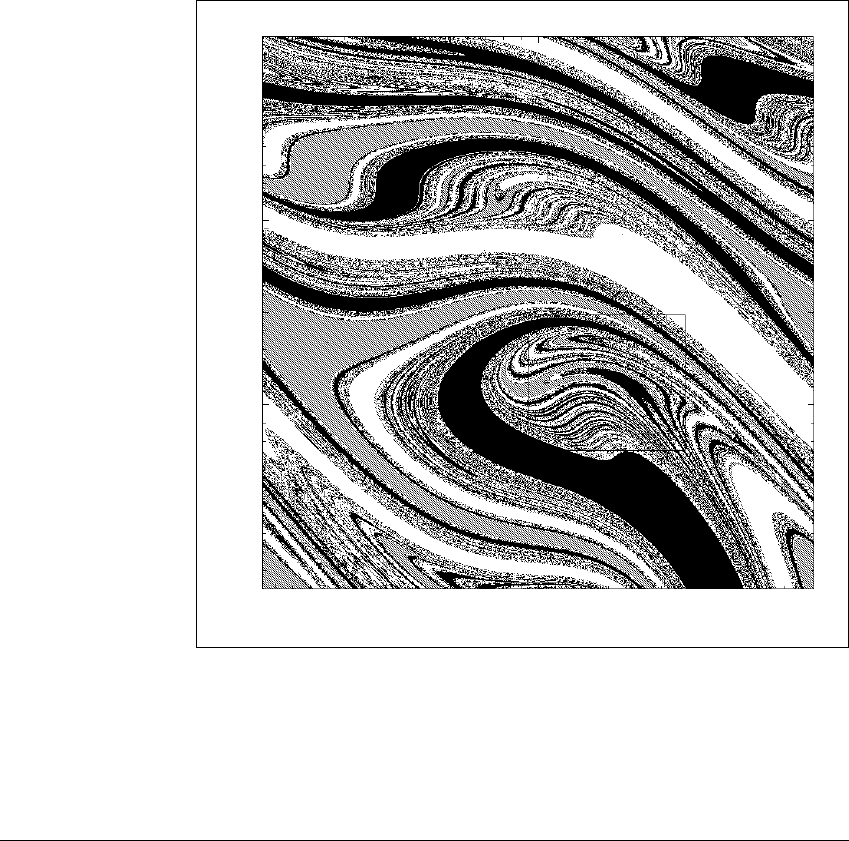
Figure 2.5 Basins of three coexisting attracting fixed points.
Parameters for the forced damped pendulum are c ⫽ 0.2,
⫽ 1.66. The basins are
shown in black, gray, and white. Each initial value (
,
˙
) is plotted according to the
sink to which it is attracted. Since the horizontal axis denotes angle in radians, the
right and left edge of the picture could be glued together, creating a cylinder. The
rectangle shown is magnified in figure 2.6.
54
2.1 MAT H E M AT IC A L M ODELS
call the forced damped pendulum model, is
¨
⫽⫺c
˙
⫺ sin
⫹
sin t. (2.10)
This differential equation includes friction (the friction constant is c)andthe
force of gravity, which pulls the pendulum bob down, as well as the sinusoidal
force
sin t, which accelerates the bob first clockwise and then counterclockwise,
continuing in a periodic way. This periodic forcing guarantees that the pendulum
will keep swinging, provided
is nonzero. The term
sin t has period 2
.
Because of the periodic forcing, if
(t) is a solution of (2.10), then so is
(t ⫹ 2
), and in fact so is
(t ⫹ 2
N) for each integer N. Assume that
(t)
is a solution of the differential equation (2.10), and define u(t) ⫽
(t ⫹ 2
).
Why is u(t) also a solution of (2.10)? Note first that
˙
u(t) ⫽
˙
(t ⫹ 2
)and
¨
u(t) ⫽
¨
(t ⫹ 2
). Second, since
(t) is assumed to be a solution for all t, (2.10)
implies
¨
(t ⫹ 2
) ⫽⫺c
˙
(t ⫹ 2
) ⫺ sin
(t ⫹ 2
) ⫹
sin(t ⫹ 2
). (2.11)
Since the nonhomogeneous term of the differential equation is periodic with
period 2
,sint ⫽ sin(t ⫹ 2
), it follows that
¨
u(t) ⫽⫺c
˙
u(t) ⫺ sin u(t) ⫹
sin t. (2.12)
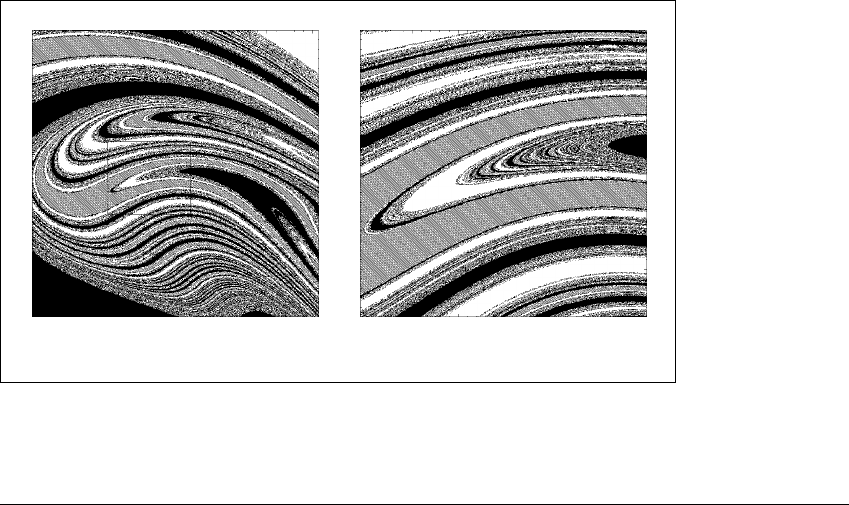
(a) (b)
Figure 2.6 Detail views of the pendulum basin.
(a) Magnification of the rectangle shown in Figure 2.5. (b) Magnification of the
rectangle shown in (a).
55

T WO-DIMENSIONAL M APS
Note that this argument depends on the fact that u (t) is a translation of
(t)by
exactly a multiple of 2
. The argument fails if we choose, for example, u(t) ⫽
(t ⫹
2) (assuming
⫽ 0).
We conclude from this fact that the time-2
map of the forced damped
pendulum is well-defined.If(
1
,
˙
1
) is the result of starting with initial conditions
(
0
,
˙
0
)attimet ⫽ 0 and following the differential equation for 2
time units,
then (
1
,
˙
1
) will also be the result of starting with initial conditions (
0
,
˙
0
)at
time t ⫽ 2
(or 4
, 6
, ...) and following the differential equation for 2
time
units. This fact allows us to study many of the important features by studying the
time-2
map of the pendulum. Because the forcing is periodic with period 2
,
the action of the differential equation is the same between 2N
and 2(N ⫹ 1)
for each integer N. Although the state equations for this system are differential
equations, we can learn a lot of information about it by viewing snapshots taken
each 2
time units.
When the pendulum is started at time t ⫽ 0, its behavior will be determined
by the initial values of
and
˙
. The differential equation uniquely determines
the values of
and
˙
at later times, such as t ⫽ 2
. If we write (
0
,
˙
0
) for the
initial values and (
1
,
˙
1
) as the values at time 2
, we can define the time-2
map F by
F(
0
,
˙
0
) ⫽ (
1
,
˙
1
). (2.13)
Just because we give the time-2
map a name does not mean that there is
a simple formula for computing it. Analyzing the time-2
map is different from
analyzing the H
´
enon map, in the sense that there is no simple expression for the
former map. The differential equation must be solved from time 0 to time 2
in order to iterate the map. For this example, investigation must be carried out
largely by computer.
Figure 2.5 shows the basins of three coexisting attractors for the time-2
map of the forced damped pendulum. Here we have set the forcing parameter
⫽ 1.66 and the damping parameter c ⫽ 0.2. The picture was made by solving
the differential equation for an initial condition representing each pixel, and
coloring the pixel white, gray, or black depending on which sink orbit attracts
the orbit.
The three attractors are one fixed point and two period-two orbits. There
are five other fixed points that are not attractors. This system displays both
great simplicity, in that the stable behaviors (sinks) are periodic orbits of low
period, and great complexity, in that the boundaries between the three basins are
infinitely-layered, or fractal.
56
2.1 MAT H E M AT IC A L M ODELS
Figure 2.6 shows further detail of the pendulum basins. Part (a) zooms in
on the rectangle in Figure 2.5; part (b) is a further magnification. Note that the
level of complication does not decrease upon magnification. The fractal structure
continues on finer and finer scales. Color Plates 3–10 show an alternate setting
of parameters for which four basins exist.
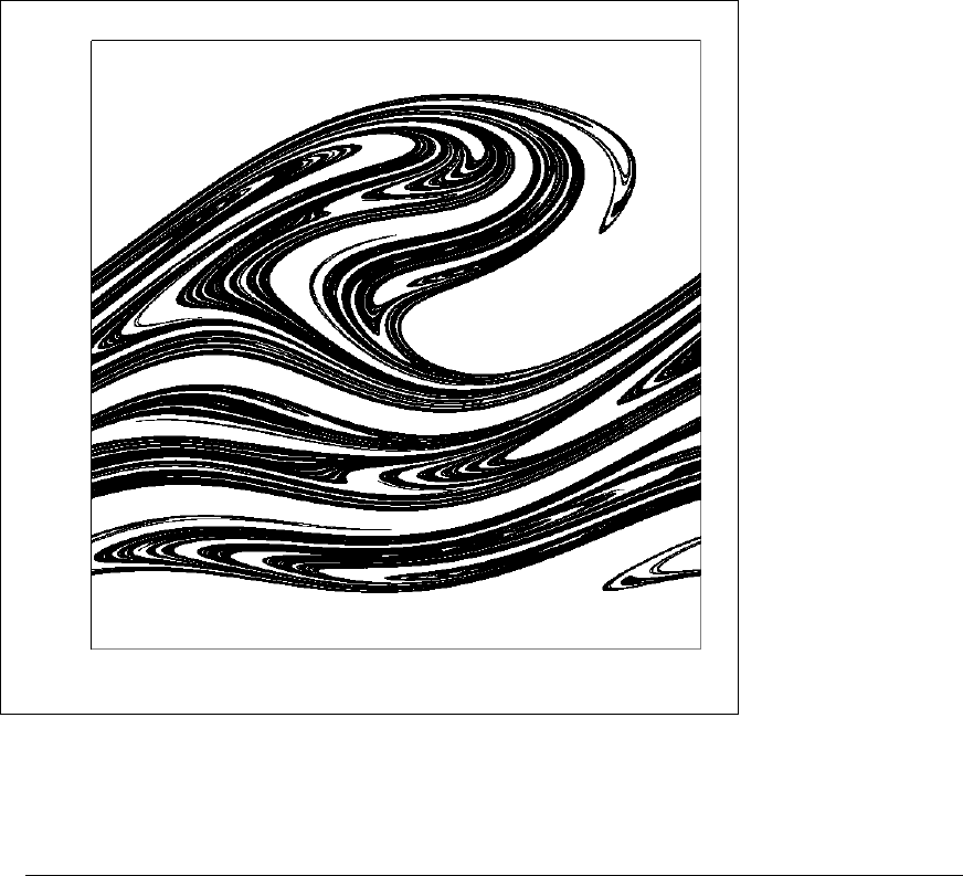
For other sets of parameter values, there are apparently no sinks for the
forced damped pendulum, fixed or periodic. Figure 2.7 shows a long orbit of the
pendulum with parameter settings c ⫽ 0.05,
⫽ 2.5. One-half million points
are shown. If these points were erased, and the next one-half million points were
plotted, the picture would look the same. There are many fixed points and periodic
orbits that coexist with this orbit. Some of them are shown in Figure 2.23(a).
4.5
⫺3.5
⫺
Figure 2.7 A single orbit of the forced damped pendulum with
c
ⴝ 0
.
05
,
ⴝ
2
.
5.
Different initial values yield essentially the same pattern, unless the initial value is
an unstable periodic orbit, of which there are several (see Figure 2.23).
57

T WO-DIMENSIONAL M APS
2.2 SINKS,SOURCES, AND SADDLES
We introduced the term “sink” in our discussion of one-dimensional maps to refer
to a fixed point or periodic orbit that attracts an
⑀
-neighborhood of initial values.
A source is a fixed point that repels a neighborhood. These definitions make sense
in higher-dimensional state spaces without alteration. In the plane, for example,
the neighborhoods in question are disks (interiors of circles).
Definition 2.1 The Euclidean length of a vector v ⫽ (x
1
,...,x
m
)in⺢
m
is |v| ⫽
x
2
1
⫹⭈⭈⭈⫹x
2
m
.Letp ⫽ (p
1
,p
2
,...,p
m
) 僆 ⺢
m
,andlet
⑀
be a positive
number. The
⑀
-neighborhood N
⑀
(p)istheset兵v 僆 ⺢
m
: |v ⫺ p| ⬍
⑀
其,theset
of points within Euclidean distance
⑀
of p. We sometimes call N
⑀
(p)an
⑀
-disk
centered at p.
Definition 2.2 Let f beamapon⺢
m
and let p in ⺢
m
be a fixed point,
that is, f(p) ⫽ p.Ifthereisan
⑀
⬎ 0 such that for all v in the
⑀
-neighborhood
N
⑀
(p), lim
k→
⬁
f
k
(v) ⫽ p,thenp is a sink or attracting fixed point.Ifthereisan
⑀
-neighborhood N
⑀
(p) such that each v in N
⑀
(p) except for p itself eventually
maps outside of N
⑀
(p), then p is a source or repeller.
Figure 2.8 shows schematic views of a sink and a source for a two-
dimensional map, along with a typical disk neighborhood and its image under
the map. Along with the sink and source, a new type of fixed point is shown in
Figure 2.8(c), which cannot occur in a one-dimensional state space. This type of
fixed point, which we will call a saddle, has at least one attracting direction and
at least one repelling direction. A saddle exhibits sensitive dependence on initial
conditions, because of the neighboring initial conditions that escape along the
repelling direction.
E XAMPLE 2.3
Consider the two-dimensional map
f(x, y) ⫽ (⫺x
2
⫹ 0.4y, x). (2.14)
This is a version of the H
´
enon map considered earlier in this chapter, with the
parameters set at a ⫽ 0andb ⫽ 0.4.
58

2.2 SINKS,SOURCES, AND S ADDLES
N
f(N)
N
f(N)
N
f(N)
(a) (b) (c)
Figure 2.8 Local dynamics near a fixed point.
The origin is (a) a sink, (b) a source, and (c) a saddle. Shown is a disk N and its
iterate under the map f.
✎ E XERCISE T2.2
Show that the map in (2.14) has exactly two fixed points, (0, 0) and
(⫺0.6, ⫺0.6).
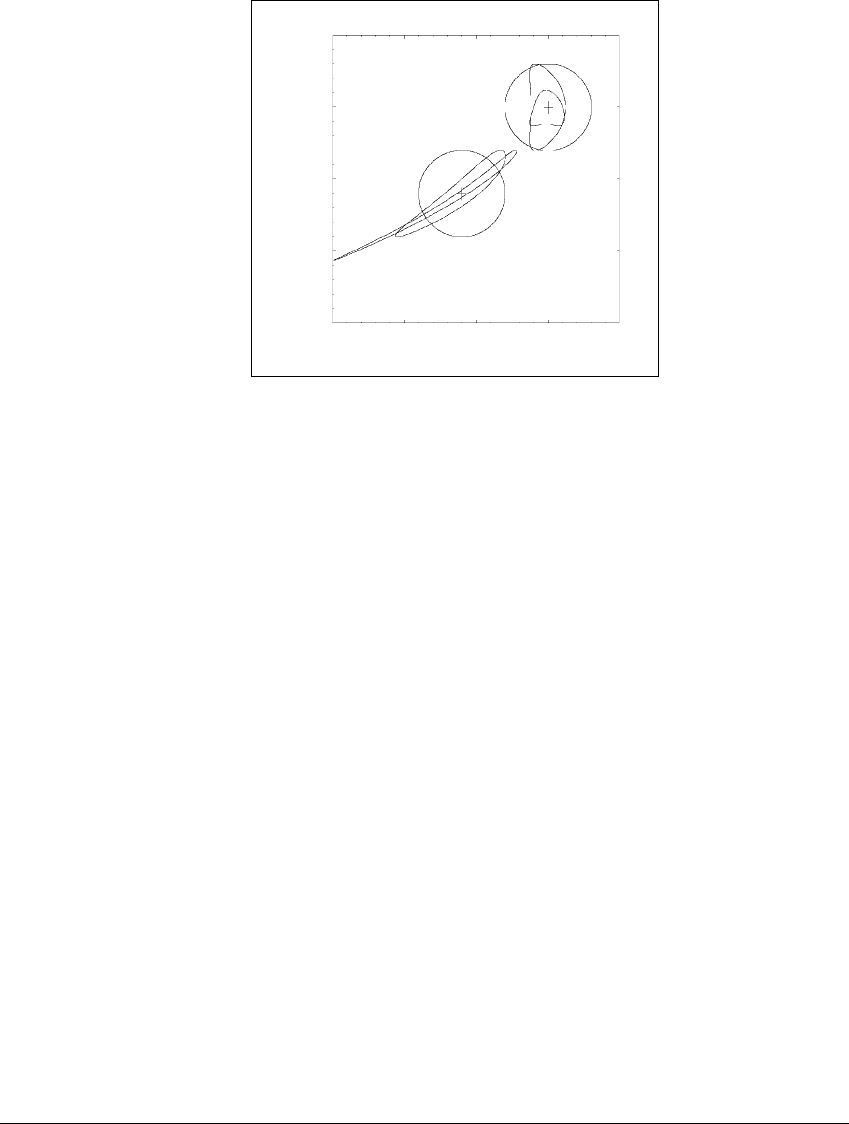
Figure 2.9 shows the two fixed points. Around each is drawn a small disk N
of radius 0. 3. Also shown are the images f(N)andf
2
(N) of each disk. The fixed
point (0, 0) is a sink, and the fixed point (⫺0.6, ⫺0.6) is a saddle. Each time the
map is iterated, the disks shrink to 40% of their previous size. Therefore f(N)is
40% the size of N,andf
2
(N) is 16% the size of N. We will explain the origin of
these numbers in Remark 2.15.
Although saddles, as well as sources, are unstable fixed points (they are
sensitive to initial conditions), they play surprising roles in the dynamics. In
Figure 2.10(a), the basin of the sink (0, 0) is shown in white. The entire square
is the box [⫺2, 2] ⫻ [⫺2, 2], and the sink is the cross at the center. Not all of
the white basin is shown: it has infinite area. The points in black diverge under
iteration by f; they are in the basin of infinity. You may wonder about the final
disposition of the points along the boundary between the two basins. Do they
go in or out? The answer is: neither. In Figure 2.10(b), the set of points that
converge to the saddle (⫺0.6, ⫺0.6) is plotted, along with the saddle denoted by
the cross. Although not an attractor, the saddle evidently plays a decisive role in
determining which points go to which basin.
59
T WO-DIMENSIONAL M APS
0.5
⫺1.5
⫺1.50.5
Figure 2.9 Local dynamics near fixed points of the H
´
enon map.
The crosses mark two fixed points of the H
´
enon map f with a ⫽ 0, b ⫽ 0.4, in the
square [⫺1.5, 0.5] ⫻ [⫺1.5, 0.5]. Around each fixed point a circle is drawn along
with its two forward images under f. On the left is a saddle: the images of the disk
are becoming increasingly long and thin. On the right the images are shrinking,
signifying a sink.
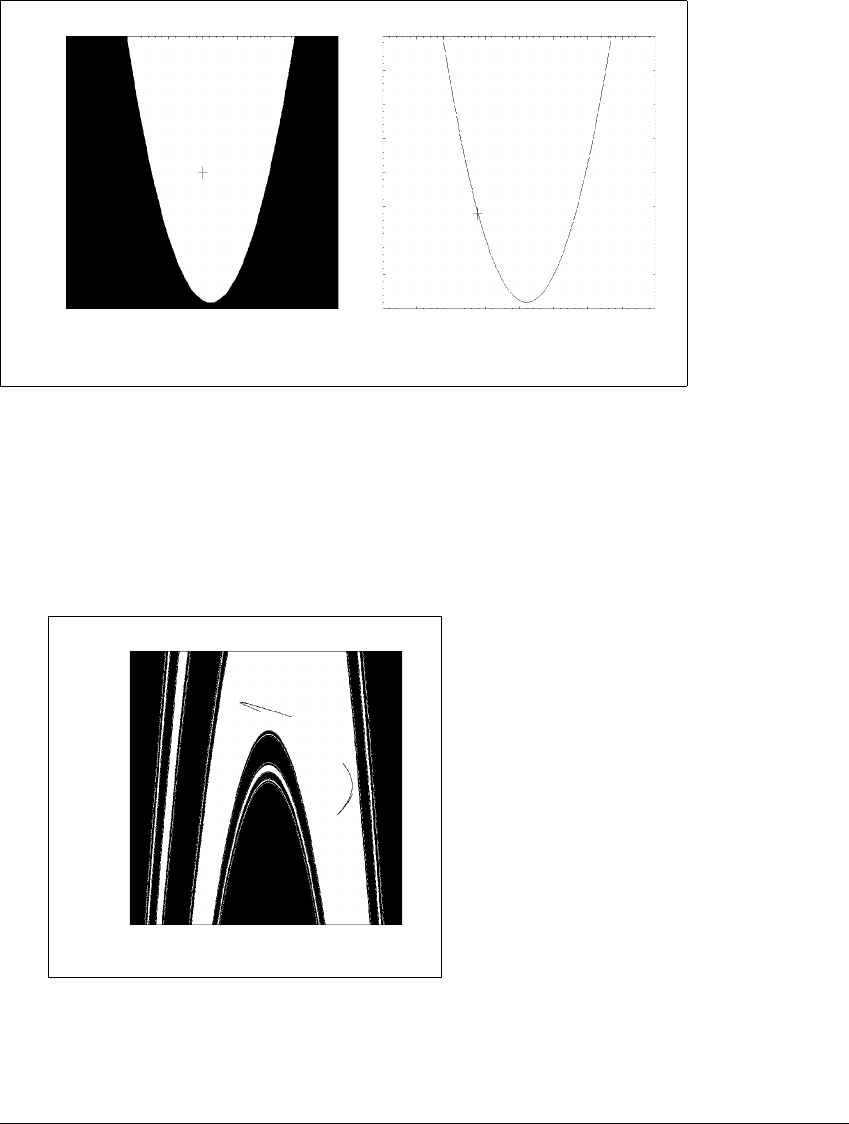
Attractors, as well as basins, can be more complicated than those shown in
Figure 2.10. Consider the H
´
enon map (2.8) with a ⫽ 2andb ⫽⫺0.3. In Figure
2.11 the dark area is again the basin of infinity, while the white set is the basin
for the two-piece attractor that looks like two hairpin curves.
Our goal in the next few sections is to find ways of identifying sinks, sources
and saddles from the defining equations of the map. In Chapter 1 we found that
the key to deciding the stability of a fixed point is the derivative at the point.
Since the derivative determines the tangent line, or best linear approximation
near the point, it determines the amount of shrinking/stretching in the vicinity
of the point. The same mechanism is operating in higher dimensions. The action
of the dynamics in the vicinity of a fixed point is governed by the best linear
approximation to the map at the point. This best linear approximation is given
by the Jacobian matrix, a matrix of partial derivatives calculated from the map.
We will define the Jacobian matrix in Section 2.5. To find out what it can tell
us, we need to fully understand linear maps first. For linear maps, the Jacobian
matrix is equal to the map itself.
60
2.2 SINKS,SOURCES, AND S ADDLES
2
⫺2
⫺22
(a)
⫺22
(b)
Figure 2.10 Basins of attraction for the H
´
enon map with
a
ⴝ 0
,b
ⴝ 0
.
4.
(a) The cross marks the fixed point (0, 0). The basin of the fixed point (0, 0) is
shown in white; the points in black diverge to infinity. (b) The initial conditions
that are on the boundary between the white and black don’t converge to (0, 0) or
infinity; instead they converge to the saddle (⫺0.6, ⫺0.6), marked with a cross.
This set of boundary points is the stable manifold of the saddle (to be discussed in
Section 2.6).
2.5
⫺2.5
⫺2.52.5
Figure 2.11 Attractors for the H
´
enon map with
a
ⴝ 2,
b
ⴝⴚ0
.
3.
Initial values in the white region are attracted to the hairpin attractor inside the
white region. On each iteration, the points on one piece of the attractor map to the
other piece. Orbits from initial values in the black region diverge to infinity.
61

T WO-DIMENSIONAL M APS
2.3 LINEAR MAPS
The linear maps on ⺢
2
are those of the particularly simple form v → Av,where
A is a 2 ⫻ 2 matrix:
A
x
y
⫽
a
11
a
12
a
21
a
22
x
y
⫽
a
11
x ⫹ a
12
y
a
21
x ⫹ a
22
y
. (2.15)
Definition 2.4 AmapA(v)from⺢
m
to ⺢
m
is linear if for each a, b 僆 ⺢,
and v, w 僆 ⺢
m
, A(av ⫹ bw) ⫽ aA(v) ⫹ bA(w). Equivalently, a linear map A(v)
can be represented as multiplication by an m ⫻ m matrix.
Every linear map has a fixed point at the origin. This is analogous to the
one-dimensional linear map f(x) ⫽ ax. The stability of the fixed point will be
investigated the same way as in Chapter 1. If all of the points in a neighborhood
of the fixed point (0, 0) approach the fixed point when iterated by the map, we
consider the fixed point to be an attractor.
In some cases the dynamics for a two-dimensional map resemble one-
dimensional dynamics. Recall that
is an eigenvalue of the matrix A if there is
a nonzero vector v such that
Av ⫽
v.
The vector v is called an eigenvector. Notice that if v
0
is an eigenvector with
eigenvalue
, we can write down a special trajectory
v
n⫹1
⫽ Av
n
that satisfies
v
1
⫽ Av
0
⫽
v
0
v
2
⫽ A
v
0
⫽
Av
0
⫽
2
v
0
,
and in general v
n
⫽
n
v
0
. Hence the map behaves like the one-dimensional map
x
n⫹1
⫽
x
n
.
We will begin by looking at three important examples of linear maps on
⺢
2
. In fact, the three different types of 2 ⫻ 2 matrices we will encounter will be
more than just good examples, they will be all possible examples, up to change of
coordinates.
62

2.3 LINEAR M APS
E XAMPLE 2.5
[Distinct real eigenvalues.] Let v ⫽ (x, y) denote a two-dimensional vector,
and let A(v)bethemapon⺢
2
defined by
A(x, y) ⫽ (ax, by).
Each input is a two-dimensional vector; so is each output. Any linear map can be
represented by multiplication by a matrix, and following tradition we use A also
to represent the matrix. Thus
A(v) ⫽ Av ⫽
a 0
0 b
x
y
. (2.16)
The eigenvalues of the matrix A are a and b, with associated eigenvectors
(1, 0) and (0, 1), respectively. For the purposes of this example, we will assume
that they are not equal, although most of what we say now will not depend on
that fact. Part of the importance of this example comes from the fact that a large
class of linear maps can be expressed in the form (2.16), if the right coordinate
system is used. For example, it is shown in Appendix A that any 2 ⫻ 2 matrix
with distinct real eigenvalues takes this form when its eigenvectors are used to
form the basis vectors of the coordinate system.
For the map in Example 2.5, the result of iterating the map n times is
represented by the matrix
A
n
⫽
a
n
0
0 b
n
. (2.17)
The unit disk is mapped into an ellipse with semi-major axes of length |a|
n
along
the x-axis and |b|
n
along the y-axis. An epsilon disk N
⑀
(0, 0) would become an
ellipse with axes of length
⑀
|a|
n
and
⑀
|b|
n
. For example, suppose that a and b are
smaller than 1 in absolute value. Then this ellipse shrinks toward the origin as
n →
⬁
,so(0, 0) is a sink for A.If|a|, |b| ⬎ 1, then the origin is a source.
On the other hand, if |a| ⬎ 1 ⬎ |b|, we see dynamical behavior that is
not seen in one-dimensional maps. As n is increased, the ellipse grows in the
x-direction and shrinks in the y-direction, essentially growing to look like the
x-axis as n →
⬁
. In Figure 2.12, we plot the unit disk and its two iterates under
A where we set a ⫽ 2andb ⫽ 1 2. In this case, the origin is neither a sink nor a
source. If the ellipses formed by successive iterates of the map grow without bound
along one direction and shrink to zero along another, we will call the origin a
saddle.
63