Alligood K., Sauer T., Yorke J.A. Chaos: An Introduction to Dynamical Systems

Подождите немного. Документ загружается.

T WO-DIMENSIONAL M APS

2.5

⫺2.5

⫺2.52.5

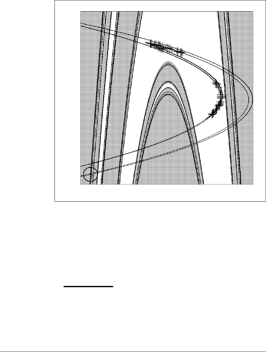
Figure 2.22 A two-piece attractor of the H

enon map.

The crosses mark 100 points of a trajectory lying on a two-piece attractor. The

basin of attraction of this attractor is white; the shaded points are initial conditions

whose orbits diverge to

⬁

. The saddle ﬁxed point circled at the lower left is closely

related to the dynamics of the attractor. The stable manifold of the saddle, shown

in black, forms the boundary of the basin of the attractor. The attractor lies along

the unstable manifold of the saddle, which is also in black.

E XAMPLE 2.23

Figure 2.23(a) shows 18 ﬁxed points (large crosses) and 38 period-two orbits

(small crosses) for the time-2

␲

map of the forced damped pendulum (2.10) with

c ⫽ 0.05,

␳

⫽ 2.5. The orbits were found by computer approximation methods;

there may be more. None of these orbits are sinks; they coexist with a complicated

attracting orbit shown in Figure 2.7. Exactly half of the 56 orbits shown are ﬂip

2.6 STA B L E AND U NSTABLE M ANIFOLDS

4.5

⫺3.5

⫺

␲␲

(a)

⫺

␲␲

(b)

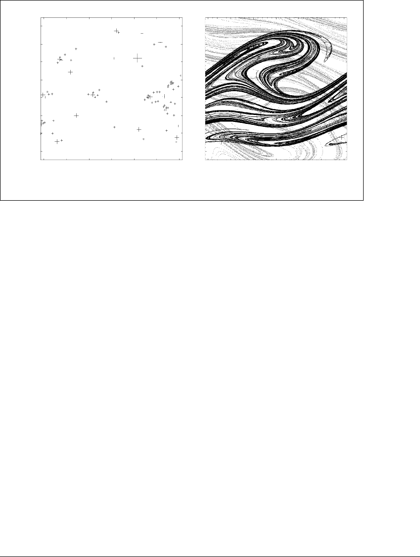
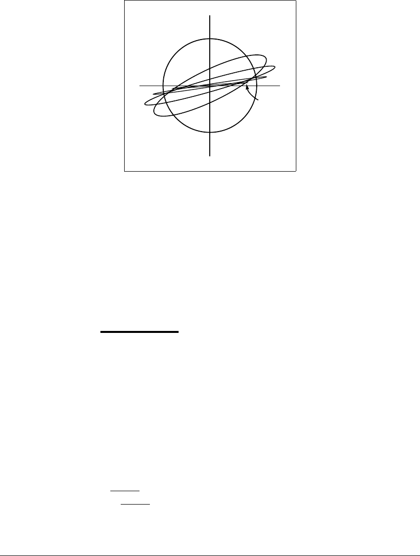
Figure 2.23 The forced damped pendulum.

(a) Periodic orbits for the time-2

␲

map of the pendulum with parameters c ⫽

0.05,

␳

⫽ 2.5. The large crosses denote 18 ﬁxed points, and the small crosses, 38

period-two orbits. (b) The stable and unstable manifolds of the largest cross in (a).

The unstable manifold is drawn in black; compare to Figure 2.7. The stable manifold

is drawn in gray dashed curves. The manifolds overlay the periodic orbits from (a)—

note that without exception these orbits lie close to the unstable manifold.

saddles; the rest are regular saddles. The largest cross in Figure 2.23(a) is singled

out, and its stable and unstable manifolds are drawn in Figure 2.23(b).

Exercise 10.6 of Chapter 10 states that a stable manifold cannot cross itself,

nor can it cross the stable manifold of another ﬁxed point. However, there is no

such restriction for a stable manifold crossing an unstable manifold.

The discovery that stable and unstable manifolds of a ﬁxed point can

intersect was made by Poincar

e. He made this observation in the process of ﬁxing

his entry to King Oscar’s contest. (In his original entry he made the assumption

that they could not cross.) Realizing this possibility was a watershed in the

knowledge of dynamical systems, whose implications are still being worked out

today.

Poincar

e was surprised to see the extreme complexity that such an inter-

section causes in the dynamics of the map. If p is a ﬁxed or periodic point, and if

⫽ p is a point of intersection of the stable and unstable manifold of p,thenh

called a homoclinic point. For starters, an intersection of the stable and unstable

manifolds of a single ﬁxed point (called a homoclinic intersection) immediately

T WO-DIMENSIONAL M APS

-1

-2

-3

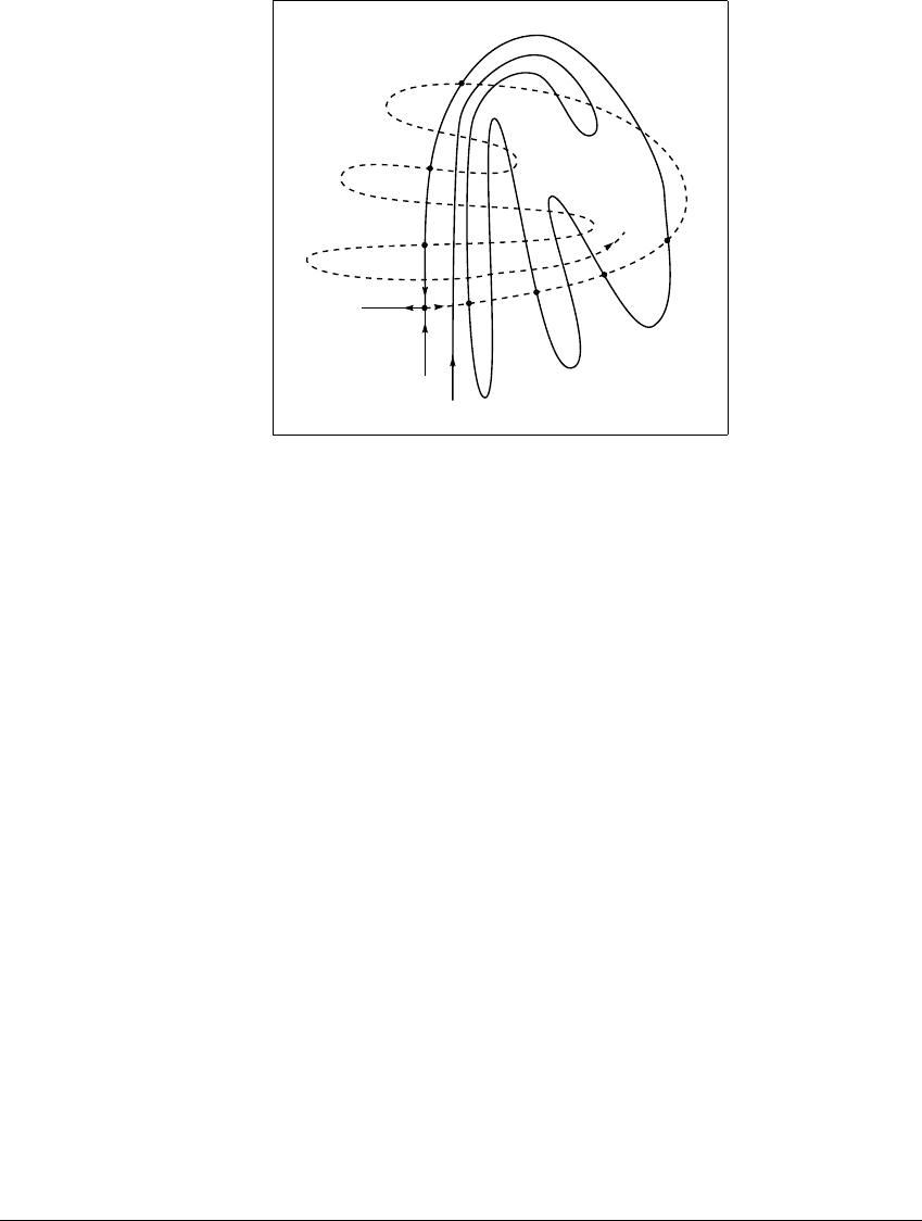
Figure 2.24 A schematic view of a homoclinic point h

The stable manifold (solid curve) and unstable manifold (dashed curve) of the

saddle ﬁxed point p intersect at h

, and therefore also at inﬁnitely many other

points. This ﬁgure only hints at the complexity. Poincar

e showed that if a circle was

drawn around any homoclinic point, there would be inﬁnitely many homoclinic

points inside the circle, no matter how small its radius.

forces inﬁnitely many such intersections. Poincar

e drew diagrams similar to Figure

2.24, which displays the inﬁnitely many intersections that logically follow from

the intersection h

To understand the source of this complexity, ﬁrst notice that a stable man-

ifold, by deﬁnition, is an invariant set under the map f. This means that if h

is a point on the stable manifold of a ﬁxed point p,thensoareh

⫽ f(h

)and

⫺1

⫽ f

⫺1

). This is easy to understand: if the orbit of h

eventually converges

to p under f, then so must the orbits of h

and h

⫺1

, being one step ahead and

behind of h

, respectively. In fact, if h

is a point on a stable manifold of p,then

so is the entire (forward and backward) orbit of h

. By the same reasoning, the

unstable manifold of a ﬁxed point is also invariant.

Once a point like h

in Figure 2.24 lies on both the stable and unstable

manifolds of a ﬁxed point, then the entire orbit of h

must lie on both manifolds,

because both manifolds are invariant. Remember that the stable manifold is

directed toward the ﬁxed point, and the unstable manifold leads away from it.

The result is a conﬁguration drawn schematically in Figure 2.24, and generated

by a computer for the H

enon map in Figure 2.21(b).

2.7 MATRIX T IMES C IRCLE E QUALS E LLIPSE

The key fact about a homoclinic intersection point is that it essentially

spreads the sensitive dependence on initial conditions—ordinarily situated at a

single saddle ﬁxed point—throughout a widespread portion of state space. Figures

2.21 and 2.24 give some insight into this process. In Chapter 10, we will return

to study this mechanism for manufacturing chaos.

2.7 MATRIX TIMES CIRCLE EQUALS ELLIPSE

Near a ﬁxed point v

, we have seen that the dynamics essentially reduce to a

single linear map A ⫽ Df(v

). If a map is linear then its action on a small disk

neighborhood of the origin is just a scaled–down version of the effect on the unit

disk. We found that the magnitudes of the eigenvalues of A were decisive for

classifying the ﬁxed point. The same is true for a period-k orbit; in that case the

appropriate matrix A is a product of k matrices.

In case the orbit is not periodic (which is one of our motivating situations),

there is no magic matrix A. The local dynamics in the vicinity of the orbit is ruled,

even in its linear approximation, by an inﬁnite product of usually nonrepeating

Df(v

). The role of the eigenvalues of A is taken over by Lyapunov numbers,

which measure contraction and expansion. When we develop Lyapunov numbers

for many-dimensional maps (Chapter 5), it is this inﬁnite product that we will

have to measure or approximate in some way.

To visualize what is going on in cases like this, it helps to have a way to

calculate the image of a disk from the matrix representing a linear map. For

simplicity, we will choose the disk of radius one centered at the origin, and a

square matrix. The image will be an ellipse, and matrix algebra explains how to

ﬁnd that ellipse.

The technique (again) involves eigenvalues. The image of the unit disk N

under the linear map A will be determined by the eigenvectors and eigenvalues

of AA

,whereA

denotes the transpose matrix of A (formed by exchanging the

rows and columns of A). The eigenvalues of AA

are nonnegative for any A.This

fact can be found in Appendix A, along with the next theorem, which shows

how to ﬁnd the explicit ellipse AN.

Theorem 2.24 Let N be the unit disk in ⺢

, and let A be an m ⫻ m matrix.

Let s

,...,s

and u

,...,u

be the eigenvalues and unit eigenvectors, respectively,

of the m ⫻ m matrix AA

. Then

1. u

,...,u

are mutually orthogonal unit vectors; and

2. the axes of the ellipse AN are s

for 1 ⱕ i ⱕ m.

T WO-DIMENSIONAL M APS

Check that in Example 2.5, the map A gives s

⫽ a, s

⫽ b, while u

and

are the x and y unit vectors, repectively. Therefore a and b are the lengths of

the axes of the ellipse AN . For the nth iterate of A, represented by the matrix A

we ﬁnd ellipse axes of length a

and b

for A

N,thenth image of the unit disk.

In Example 2.5, the axes of the ellipse AN are easy to ﬁnd. Each axis is an

eigenvector not only of AA

but also of A, whose length is the corresponding

eigenvalue of A. In general (for nonsymmetric matrices), the eigenvectors of A

do not give the directions along which the ellipse lies, and it is necessary to use

Theorem 2.24. To see how Theorem 2.24 applies in general, we’ll return for a

look at our three important examples.

E XAMPLE 2.25

[Distinct real eigenvalues.] Let

A(x) ⫽ Ax ⫽



.8 . 5

01.3





. (2.36)

The eigenvalues of the matrix A are 0.8and1.3, with corresponding eigenvectors





and





, respectively. From this it is clear that the ﬁxed point at the origin

is a saddle—the two eigenvectors give directions along which the ﬁxed point

attracts and repels, respectively. The attracting direction is illustrated by





⫽ (0.8)





⫽



(0.8)



, (2.37)

and the repelling direction by





⫽ (1.3)





⫽



(1.3)



. (2.38)

The stable manifold of the origin saddle point is y ⫽ 0, and the unstable manifold

is y ⫽ x. Points along the x-axis move directly toward the origin under iteration

by A, and points along the line y ⫽ x move toward inﬁnity. Since we know the

nth iterate of the unit circle is an ellipse with one growing direction and one

shrinking direction, we know that in the limit the ellipses become long and thin.

The ellipses A

N representing higher iterates of the unit disk gradually line up

along the dominant eigenvector





of A.

The ﬁrst few images of the unit disk under the map A can be found using

Theorem 2.24, and are graphed in Figure 2.25. For an application of Theorem

2.7 MATRIX T IMES C IRCLE E QUALS E LLIPSE

-2

-3

-4

-5

-4 -3 -2

y = x

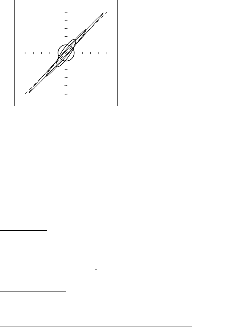
Figure 2.25 Successive images of the unit circle

for a saddle ﬁxed point.

The image of a circle under a linear map is an ellipse. Successive images are therefore

also ellipses, which in this example line up along the expanding eigenspace.

2.24, we calculate the ﬁrst iterate of the unit disk under A.Since

⫽



.8 . 5

01.3



.80

.51.3



⫽



.89 .65

.65 1.69



, (2.39)

the unit eigenvectors of AA

are (approximately)



.873

⫺.488



and



.488

.873



,with

eigenvalues .527 and 2.053, respectively. Taking square roots, we see that the

ellipse AN has principal axes of lengths ⬇



.527 ⬇ .726 and ⬇



2.053 ⬇

1.433. The ellipse AN, along with A

N and A

N, is illustrated in Figure 2.25.

E XAMPLE 2.26

[Repeated eigenvalue.] Even in the sink case, the ellipse A

N can grow a

little in some direction before shrinking for large n. Consider the example

A ⫽





. (2.40)

✎ E XERCISE T2.10

Use Theorem 2.24 to calculate the axes of the ellipse AN from (2.40). Then

verify that the ellipses A

N shrink to the origin as n →

⬁

T WO-DIMENSIONAL M APS

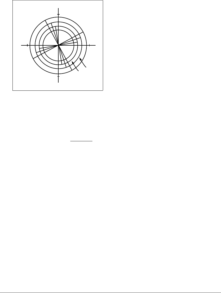
Figure 2.26 Successive images of the unit circle

under a linear map

the case of repeated eigenvalues.

The nth iterate A

N of the circle lies wholly inside the circle for n ⱖ 6. In this case,

the origin is a sink.

The ﬁrst few iterates of the unit circle N are graphed in Figure 2.26. The

ellipse AN sticks out of the unit disk N. Further iteration by A continues to roll

the ellipse to lie parallel to the x-axis and to eventually shrink it to the origin, as

the calculation of Exercise T2.10 requires.

E XAMPLE 2.27

[Complex eigenvalues.] Let

A ⫽



a ⫺b



. (2.41)

The eigenvalues of this matrix are a ⫾ bi. Calculating AA

yields

⫽



⫹ b

0 a

⫹ b



, (2.42)

so it follows that the image of the unit disk N by A is again a disk of radius



⫹ b

. The matrix A rotates the disk by arctan b a and stretches by a factor



⫹ b

on each iteration. The stability result is the same as in the previous

two cases: if the absolute value of the eigenvalues is less than 1, the origin is a

sink; if greater than 1, a source.

2.7 MATRIX T IMES C IRCLE E QUALS E LLIPSE

2-2

-2

Figure 2.27 Successive images of the unit circle

The origin is a source with complex eigenvalues.

In Figure 2.27, the ﬁrst few iterates A

N of the unit disk are graphed for

a ⫽ 1.2,b⫽ 0.2. Since a

⫹ b

⬎ 1, the origin is a source. The radii of the images

of the disk grow at the rate of



1.2

⫹ .2

⬇ 1.22 per iteration, and the disks

turn counterclockwise at the rate of arctan(.2 1.2) ⬇ 9.5 degrees per iteration.

8:36 pm, 4/30/05

T WO-DIMENSIONAL M APS

☞ C HALLENGE 2

Counting the Periodic Orbits of Linear Maps

on a Torus

N CHAPTER 1, we investigated the properties of the linear map f(x) ⫽ 3x

(mod 1). This map is discontinuous on the interval [0, 1], but continuous when

viewed as a map on a circle. We found that the map had inﬁnitely many periodic

points, and we discussed ways to count these orbits.

We will study a two-dimensional map with some of the same properties in

Challenge 2. Consider the map S deﬁned by a 2 ⫻ 2 matrix

A ⫽





with integer entries a, b, c, d, where we deﬁne S(v) ⫽ Av (mod 1). The domain

for the map will be the unit square [0, 1] ⫻ [0, 1]. Even if Av lies outside the

unit square, S(v) lies inside if we count modulo one. In general, S will fail to be

continuous, in the same way as the map in Example 1.9 of Chapter 1.

For example, assume

A ⫽





. (2.43)

Consider the image of the point v ⫽ (x, 1 2) under S. For x slightly less than

1 2, the image S(v) lies just below (1 2, 1). For x slightly larger than 1 2, the

image S(v) lies just above (1 2, 0), quite far away. Therefore S is discontinuous

at (1 2, 1 2).

We solved this problem for the 3x mod 1 map in Chapter 1 by sewing

together the ends of the unit interval to make a circle. Is there a geometric object

for which S can be made continuous? The problem is that when the image value

1 is reached (for either coordinate x or y), the map wants to restart at the image

value 0.

The torus ⺤

is constructed by identifying the two pairs of opposite sides

of the unit square in ⺢

. This results in a two-dimensional object resembling

a doughnut, shown in Figure 2.28. We have simultaneously glued together the

x-axis at 0 and 1, and the y-axis at 0 and 1. The torus is the natural domain for

maps that are formed by integer matrices modulo one.

C HALLENGE 2

(a) (b) (c)

Figure 2.28 Construction of a torus in two easy steps.

(a) Begin with unit square. (b) Identify (glue together) vertical sides. (c) Identify

horizontal sides.

Given a 2 ⫻ 2 matrix A, we can deﬁne a map from the torus to itself by

multiplying the matrix A times a vector (x, y), followed by taking the output

vector modulo 1. If the matrix A has integer entries, then the map so deﬁned

is continuous on the torus. In the following steps we derive some fundamental

properties of torus maps, and then specialize to the particular map (2.43), called

the cat map.

Assume in Steps 1–6 that A has integer entries, and that the determinant

of A, det(A) ⫽ ad ⫺ bc, is nonzero.

Step 1 Show that the fact that A is a 2 ⫻ 2 matrix with integer entries

implies that the torus map S(v) ⫽ Av (mod 1) is a continuous map on the torus

⺤

. (You will need to explain why the points (0,y)and(1,y), which are identiﬁed

together on the torus, map to the same point on the torus. Similarly for (x, 0) and

(x, 1).)

Step 2 (a) Show that A



x ⫹ n

y ⫹ n



⫽ A





(mod 1) for any integers

(b) Show that S

(v) ⫽ A

v (mod 1).

(v) ⫽ A

v (mod 1) for any positive integer n.

Step 2 says that in computing the nth iterate of S, you can wait until the

end to apply the modulo 1 operation.

A real number r is rational if r ⫽ p q,wherep and q are integers. A number

that is not rational is called irrational. Note that the sum or product of two

rational numbers is rational, the sum of a rational and an irrational is irrational,