Alligood K., Sauer T., Yorke J.A. Chaos: An Introduction to Dynamical Systems

Подождите немного. Документ загружается.

T WO-DIMENSIONAL M APS

2.5

⫺2.5

01.25

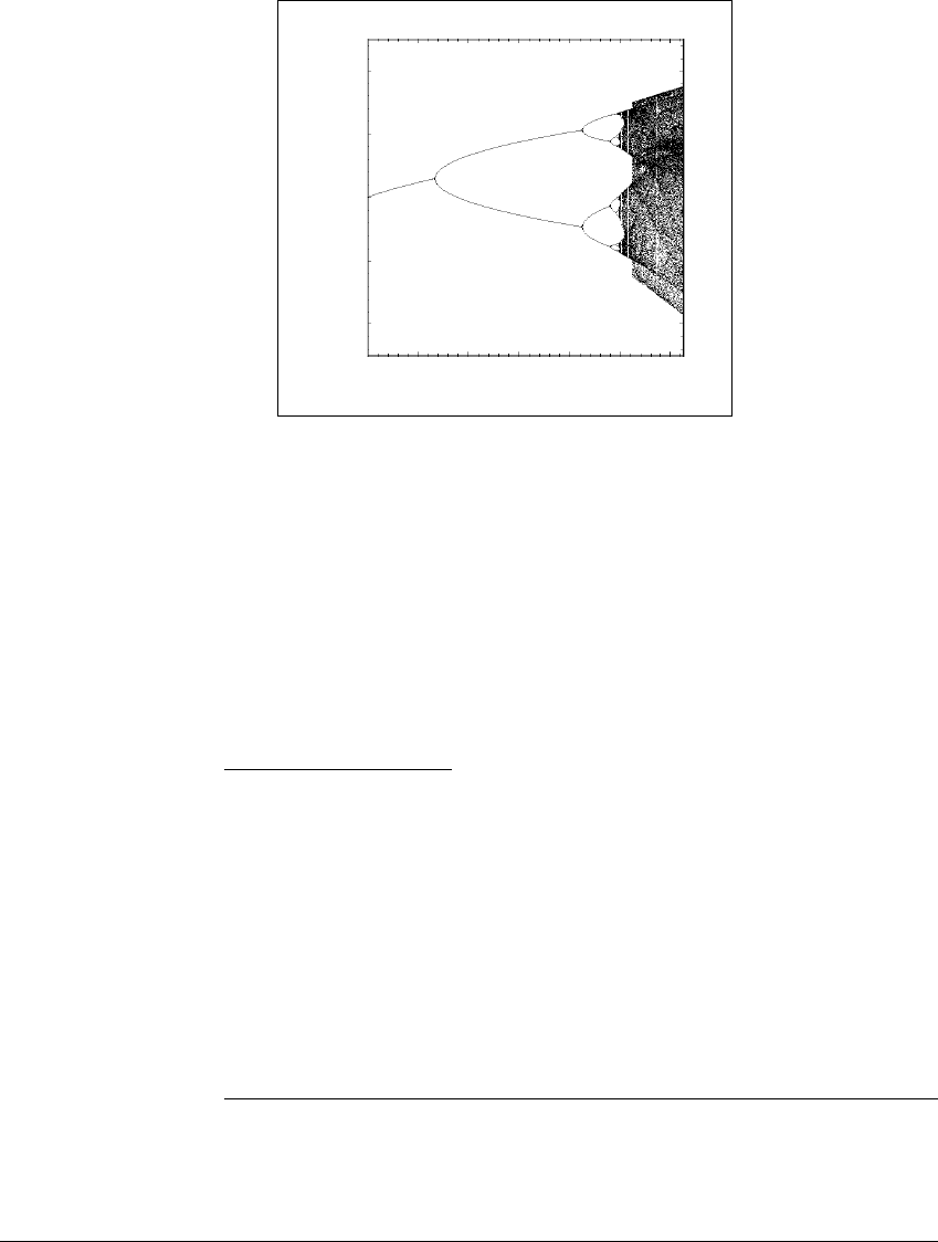
Figure 2.16 Bifurcation diagram for the H

enon map,

ⴝ 0

Each vertical slice shows the projection onto the x-axis of an attractor for the map

for a ﬁxed value of the parameter a.

2.15 is recapitulated here. At a ⫽ 0.27, a period-doubling bifurcation occurs,

when the ﬁxed point loses stability and a period-two orbit is born. The period-

two orbit is a sink until a ⫽ 0.85, when it too doubles its period. In the next

exercise, you will be asked to use the equations we developed here to verify some

of these facts.

✎ E XERCISE T2.7

Set b ⫽ 0.4.

(a) Prove that for ⫺0.09 ⬍ a ⬍ 0.27, the H

enon map f has one sink

ﬁxed point and one saddle ﬁxed point.

(b) Find the largest magnitude eigenvalue of the Jacobian matrix at

the ﬁrst ﬁxed point when a ⫽ 0.27. Explain the loss of stability of the sink.

(d) Find the largest magnitude eigenvalue of Df

, the Jacobian of f

at the period-two orbit, when a ⫽ 0.85.

For b ⫽ 0.4anda ⬎ 0.85, the attractors of the H

enon map become more

complex. When the period-two orbit becomes unstable, it is immediately replaced

with an attracting period-four orbit, then a period-eight orbit, etc. Figure 2.17

2.5 NONLINEAR M APS AND THE J ACOBIAN M ATRIX

Figure 2.17 Attractors for the H

enon map with

ⴝ 0

Each panel displays a single attracting orbit for a particular value of the parameter

a.(a)a ⫽ 0.9, period 4 sink. (b) a ⫽ 0.988, period 16 sink. (c) a ⫽ 1.0, four-piece

attractor. (d) a ⫽ 1.0293, period-ten sink. (e) a ⫽ 1.045, two-piece attractor. The

points of an orbit alternate between the pieces. (f) a ⫽ 1.2, two pieces have merged

to form one-piece attractor.

T WO-DIMENSIONAL M APS

shows a number of these attractors. An example is the “period-ten window” at

a ⫽ 1.0293, barely detectable as a vertical white gap in Figure 2.16.

➮ COMPUTER EXPERIMENT 2.2

Make a bifurcation diagram like Figure 2.16, but for b ⫽⫺0.3, and for

0 ⱕ a ⱕ 2.2. For each a, choose the initial point (0, 0) and calculate its orbit.

Plot the x-coordinates of the orbit, starting with iterate 101 (to allow time for the

orbit to approximately settle down to the attracting orbit). Questions to answer:

Does the resulting bifurcation diagram depend on the choice of initial point? How

is the picture different if the y-coordinates are plotted instead?

Periodic points are the key to many of the properties of a map. For example,

trajectories often converge to a periodic sink. Periodic saddles and sources, on the

other hand, do not attract open neighborhoods of initial values as sinks do, but

are important in their own ways, as will be seen in later chapters.

Remark 2.15 The theme of this section has been the use of the Jacobian

matrix for determining stability of periodic orbits of nonlinear maps, in the way

that the map matrix itself is used for linear maps. There are other important

uses for the Jacobian matrix. The magnitude of its determinant measures the

transformation of areas for nonlinear maps, at least locally.

For example, consider the H

enon map (2.27). The determinant of the

Jacobian matrix (2.28) is ﬁxed at ⫺b for all v. For the case a ⫽ 0,b ⫽ 0.4, the

map f transforms area near each point v at the rate |det(Df(v))| ⫽ | ⫺ b| ⫽ 0.4.

Each plane region is transformed by f into a region that is 40% of its original size.

The circle around each ﬁxed point in Figure 2.9, for example, has forward images

which are .4 ⫽ 40% and (.4)

⫽ .16 ⫽ 16%, respectively.

Most of the plane maps we will deal with are invertible, meaning that their

inverses exist.

Deﬁnition 2.16 Amapf on ⺢

is one-to-one if f(v

) ⫽ f(v

) implies

⫽ v

Recall that functions are well-deﬁned by deﬁnition, i.e. v

⫽ v

implies

f(v

) ⫽ f(v

). Two points do not get mapped together under a one-to-one map.

It follows that if f is a one-to-one map, then its inverse map f

⫺1

is a function. The

2.5 NONLINEAR M APS AND THE J ACOBIAN M ATRIX

INVERSE MAPS

A function is a uniquely-deﬁned assignment of a range point for each

domain point. (If the domain and range are the same set, we call the

function a map.) Several domain points may map to the same range

point. For f

(x, y) ⫽ (x

), the points (2, 2), (2, ⫺2), (⫺2, 2) and

(⫺2, ⫺2) all map to (4, 4). On the other hand, for f

(x, y) ⫽ (x

this never happens. A point (a, b) is the image of (a

1 3

)only.

Thus f

is a one-to-one map, and f

is not.

An inverse map f

⫺1

automatically exists for any one-to-one map f.

The domain of f

⫺1

is the image of f. For the example f

(x, y) ⫽

), the inverse is f

⫺1

(x, y) ⫽ (x

1 3

To compute an inverse map, set v

⫽ f(v) and solve for v in terms of

. We demonstrate using f(x, y) ⫽ (x ⫹ 2y, x

). Set

⫽ x ⫹ 2y

⫽ x

and solve for x and y. The result is

x ⫽ y

1 3

y ⫽ (x

⫺ y

1 3

) 2,

so that the inverse map is f

⫺1

(x, y) ⫽ (y

1 3

, (x

⫺ y

1 3

) 2).

inverse map is characterized by the fact that f(v) ⫽ w if and only if v ⫽ f

⫺1

(w).

Because one-to-one implies the existence of an inverse, a one-to-one map is also

called an invertible map.

✎ E XERCISE T2.8

Show that the H

enon map (2.27) with b ⫽ 0 is invertible by ﬁnding a formula

for the inverse. Is the map one-to-one if b ⫽ 0?

T WO-DIMENSIONAL M APS

2.6 STABLE AND UNSTABLE MANIFOLDS

A saddle ﬁxed point is unstable, meaning that most initial values near it will

move away under iteration of the map. However, unlike the case of a source, not

all nearby initial values will move away. The set of initial values that converge to

the saddle will be called the stable manifold of the saddle. We start by looking at

a simple linear example.

E XAMPLE 2.17

For the linear map f(x, y) ⫽ (2x, y 2), the origin is a saddle ﬁxed point.

The dynamics of this map were shown in Figure 2.14. It is clear from that ﬁgure

that points along the y-axis converge to the saddle 0; all other points diverge to

inﬁnity. Unless the initial value has x-coordinate 0, the x-coordinate will grow

(by a factor of 2 per iterate) and get arbitrarily large.

A convenient way to view the direction of the stable manifold in this case

is in terms of eigenvectors. The linear map

f(v) ⫽ A v ⫽



00.5





has eigenvector





, corresponding to the (stretching) eigenvalue 2, and





corresponding to the (shrinking) eigenvalue 1 2. The latter direction, the y-axis,

is the “incoming” direction, and is the stable manifold of 0. We will call the x-axis

the “outgoing” direction, the unstable manifold of 0. Another way to describe

the unstable manifold in this example is as the stable manifold under the inverse

of the map f

⫺1

(x, y) ⫽ ((1 2)x, 2y).

Deﬁnition 2.18 Let f be a smooth one-to-one map on ⺢

, and let p

be a saddle ﬁxed point or periodic saddle point for f.Thestable manifold of p,

denoted

S(p), is the set of points v such that |f

(v) ⫺ f

(p)| → 0 as n →

⬁

The unstable manifold of p, denoted

U(p), is the set of points v such that

⫺n

(v) ⫺ f

⫺n

(p)| → 0 as n →

⬁

E XAMPLE 2.19

The linear map f(x, y) ⫽ (⫺2x ⫹

y, ⫺5x ⫹

y) has a saddle ﬁxed point

at 0 with eigenvalues 0.5 and 3. The corresponding eigenvectors are (1, 1) and

2.6 STA B L E AND U NSTABLE M ANIFOLDS

W HAT IS A M ANIFOLD?

n n-dimensional manifold is a set that locally resembles Euclidean

space ⺢

. By “resembles” we could mean a variety of things, and

in fact, various deﬁnitions of manifold have been proposed. For our

present purposes, we will mean resemblance in a topological sense. A

small piece of a manifold should look like a small piece of ⺢

A 1-dimensional manifold is locally a curve. Every short piece of a

curve can be formed by stretching and bending a piece of a line. The

letters D and O are 1-manifolds. The letters A and X are not, since

each contains a point for which no small neighborhood looks like a

line segment. These bad points occur at the meeting points of separate

segments, like the center of the letter X.

Notable 2-manifolds are the surface of oranges and doughnuts. The

space-time continuum of the universe is often described as a 4-

manifold, whose curvature due to relativity is an active topic among

cosmologists.

In the strict deﬁnition of manifold, each point of a manifold must

have a neighborhood around itself that looks like ⺢

. Thus the letters

L and U fail to be 1-manifolds because of their endpoints—small

neighborhoods of them look like a piece of half-line (say the set of

nonnegative real numbers), not a line, since there is nothing on one

side. This type of set is called a manifold with boundary, although

technically it is not a manifold. A M

obius band is a 2-manifold with

boundary because the edge looks locally like a piece of half-plane,

not a plane. Whole oranges and doughnuts are 3-manifolds with

boundary.

One of the goals of Chapter 10 is to explain why a stable or unstable

manifold is a topological manifold. Stable and unstable manifolds

emanate from two opposite sides of a ﬁxed point or periodic orbit. At

a saddle point in the plane, they together make an “X” through the

ﬁxed point, although individually they are manifolds.

T WO-DIMENSIONAL M APS

(1, 2), respectively. [According to Appendix A, there is a linear change of coor-

dinates giving the map h(u

) ⫽ (0.5u

, 3u

).] Points lying on the line y ⫽ x

undergo the dynamics v → 0.5v on each iteration of the map. This line is the

stable manifold of 0 for f. Points lying on the line y ⫽ 2x (the line in the direc-

tion of eigenvector (1, 2)) undergo v → 3v under f: this is the unstable manifold.

These sets are illustrated in Figure 2.18.

E XAMPLE 2.20

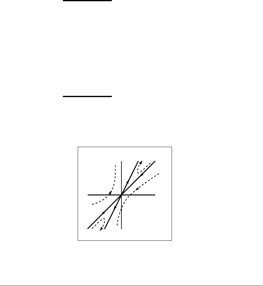
Let f(x, y) ⫽ (2x ⫹ 5y, ⫺0.5y). The eigenvalues of f are 2 and ⫺0.5, with

corresponding eigenvectors (1, 0) and (2, ⫺1). Points on the line in the direction

of the vector (2, ⫺1) undergo v → ⫺0.5v on each iteration of f. As a result,

successive images ﬂip from one side of the origin to the other along the line. This

ﬂipping behavior of orbits about the ﬁxed point is shown in Figure 2.19. It is

characteristic of all ﬁxed points for which the Jacobian has negative eigenvalues,

even when the map is nonlinear. A saddle with at least one negative eigenvalue

is sometimes called a ﬂip saddle. Otherwise it is a regular saddle.

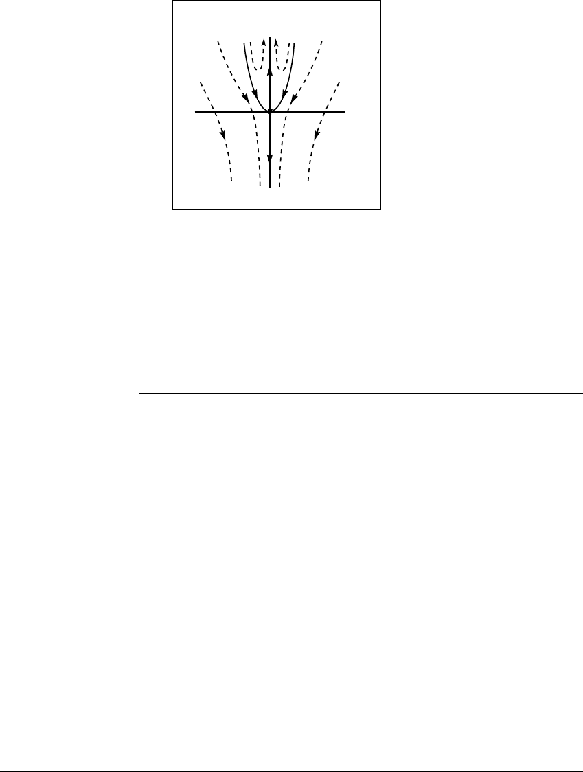
E XAMPLE 2.21

The invertible nonlinear map f(x, y) ⫽ (x 2, 2y ⫺ 7x

) has a ﬁxed point

at 0 ⫽ (0, 0). To analyze the stability of this ﬁxed point we evaluate

Figure 2.18 Stable and unstable manifolds for regular saddle.

The stable manifold is the solid inward-directed line; the unstable manifold is the

solid outward-directed line. Every initial condition leads to an orbit diverging to

inﬁnity except for the stable manifold of the origin.

2.6 STA B L E AND U NSTABLE M ANIFOLDS

Figure 2.19 Stable and unstable manifolds for ﬂip saddle.

Flipping occurs along the stable manifold (inward-directed line). The unstable

manifold is the x-axis.

Df(0, 0) ⫽



0.50



The origin is a saddle ﬁxed point. The eigenvectors lie on the two coordinate axes.

What is the relation of these eigenvector directions to the stable and unstable

manifolds?

In the case of linear maps, the stable and unstable manifolds coincide with

the eigenvector directions. For a saddle of a general nonlinear map, the stable

manifold is tangent to the shrinking eigenvector direction, and the unstable man-

ifold is tangent to the stretching eigenvector direction. Since f(0,y) ⫽ (0, 2y),

the y-axis can be seen to be part of the unstable manifold. For any point not on

the y-axis, the absolute value of the x-coordinate is nonzero and increases under

iteration by f

⫺1

; in particular, it doesn’t converge to the origin. Thus the y-axis is

the entire unstable manifold, as shown in Figure 2.20. The stable manifold of 0,

however, is described by the parabola y ⫽ 4x

; i.e., S(0) ⫽ 兵(x, 4x

):x 僆⺢其.

✎ E XERCISE T2.9

Considerthesaddleﬁxedpoint0 of the map f(x, y) ⫽ (x 2, 2y ⫺ 7x

)from

Example 2.21.

(a) Find the inverse map f

⫺1

(b) Show that the set

S ⫽ 兵(x, 4x

):x 僆⺢其 is invariant under f,that

is, if v is in S,thenf(v)andf

⫺1

(v)areinS.

T WO-DIMENSIONAL M APS

Figure 2.20 Stable and unstable manifolds for the nonlinear map of Example

2.21.

The stable manifold is a parabola tangent to the x-axis at 0; the unstable manifold

is the y-axis.

(d) Show that no points outside of

S converge to 0 under f.

When a map is linear, the stable and unstable manifolds of a saddle are

always linear subspaces. In the case of linear maps on ⺢

, for example, they are

lines. For nonlinear maps, as we saw in Example 2.21, they can be curves. The

nonlinear examples we have looked at so far are not typical; usually, formulas

for the stable and unstable manifolds cannot be found directly. Then we must

rely on computational techniques to approximate their locations. (We describe

one such technique in Chapter 10.) One thing you may have noticed about the

stable manifolds in these examples is that they are always one-dimensional: lines

or curves. Just as in the linear case, the stable and unstable manifolds of saddles in

the plane are always one-dimensional sets. This fact is not immediately obvious—

it is proved as part of the Stable Manifold Theorem in Chapter 10. We will also

see that stable and unstable manifolds of saddles have a tremendous inﬂuence on

the underlying dynamics of a system. In particular, their relative positions can

determine whether or not chaos occurs.

We will leave the investigation of the mysteries of stable and unstable

manifolds to Chapter 10. Here we give a small demonstration of the subtlety

and importance of these manifolds. Drawing stable and unstable manifolds of the

enon map can illuminate Figure 2.3, which showed the basin of the period-two

2.6 STA B L E AND U NSTABLE M ANIFOLDS

2.5

⫺2.5

⫺2.52.5

(a)

⫺2.52.5

(b)

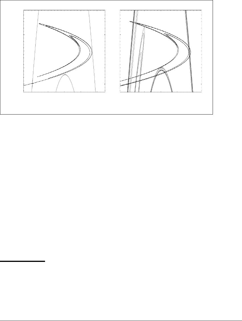
Figure 2.21 Stable and unstable manifolds for a saddle point.

The stable manifolds (mainly vertical) and unstable manifolds (more horizontal)

are shown for the saddle ﬁxed point (marked with a cross in the lower left corner) of

the H

enon map with b ⫽⫺0.3. Note the similarity of the unstable manifold with

earlier ﬁgures showing the H

enon attractor. (a) For a ⫽ 1.28, the leftward piece of

the unstable manifold moves off to inﬁnity, and the rightward piece initially curves

toward the sink, but oscillates around it in an erratic way. The rightward piece is

contained in the region bounded by the two components of the stable manifold.

(b) For a ⫽ 1.4, the manifolds have crossed one another.

sink under two different parameter settings. In Figure 2.21, portions of the stable

and unstable manifolds of a saddle point near (⫺2, ⫺2) are drawn. In each case,

the upward and downward piece of the stable manifold, which is predominantly

vertical, forms the boundary of the basin of the period-two sink. (Compare with

Figure 2.3.) For a larger value of the parameter a, as in Figure 2.21(b), the stable

and unstable manifolds intersect, and the basin boundary changes from simple to

complicated.

E XAMPLE 2.22

Figure 2.22 shows the relation of the stable and unstable manifolds to the

basin of the two-piece attractor for the H

enon map with a ⫽ 2, b ⫽⫺0.3. This

basin was shown earlier in Figure 2.11. The stable manifold of the saddle ﬁxed

point in the lower left corner forms the boundary of the attractor basin; the

attractor lies along the unstable manifold of the saddle.