Alligood K., Sauer T., Yorke J.A. Chaos: An Introduction to Dynamical Systems

Подождите немного. Документ загружается.

T WO-DIMENSIONAL M APS

2.1 MATHEMATICAL MODELS

Maps are important because they encode the behavior of deterministic systems.

We have discussed population models, which have a single input (the present

population) and a single output (next year’s population). The assumption of

determinism is that the output can be uniquely determined from the input.

Scientists use the term “state” for the information being modeled. The state of

the population model is given by a single number—the population—and the state

space is one-dimensional. We found in Chapter 1 that even a model where the

state runs along a one-dimensional axis, as G(x) ⫽ 4x(1 ⫺ x), can have extremely

complicated dynamics.

The changes in temperature of a warm object in a cool room can be modeled

as a one-dimensional map. If the initial temperature difference between the object

and the room is D(0), the temperature difference D(t)aftert minutes is

D(t) ⫽ D(0)e

⫺Kt

, (2.1)

where K ⬎ 0 depends on the speciﬁc heat of the object. We can call the model

f(x) ⫽ e

⫺K

x (2.2)

the “time-1 map”, because application of this map advances the system one

minute. Since e

⫺K

is a constant, f is a linear one-dimensional map, the easiest

type we studied in Chapter 1. It is clear that the ﬁxed point x ⫽ 0 is a sink because

⫺K

| ⬍ 1. More generally, we could consider the map that advances the system

T time units, the time-T map. For any ﬁxed time T,thetime-T map for this

example is the linear one-dimensional map f(x) ⫽ e

⫺KT

x, also written as

x −→ e

⫺KT

x. (2.3)

Formula (2.1) is derived from Newton’s law of cooling, which is the differ-

ential equation

⫽⫺kD, (2.4)

with initial value D(0). There is a basic assumption that the body is a good

conductor so that at any instant, the temperature throughout the body is uniform.

Equation (2.3) is an example of the derivation of a map as the time-T map of a

differential equation.

In the examples above, the state space is one-dimensional, meaning that

the information needed to advance the model in time is a single number. This is in

effect the deﬁnition of state in mathematical modeling: the amount of information

2.1 MAT H E M AT IC A L M ODELS

needed to advance the model. Nothing else is relevant for the purposes of the

model, so the state is completely sufﬁcient to describe the conditions of the system.

In the case of a one-dimensional map or a single differential equation, the state is

a single number. In the case of a two-dimensional map or a system of two coupled

ordinary differential equations, it is a pair of numbers. The state is essentially

the initial information needed for the dynamical system model to operate and

respond unambiguously with an orbit. In partial differential equations models, the

state space may be inﬁnite-dimensional. In such a case, inﬁnitely many numbers

are needed to specify the current state. For a vibrating string, modeled by a partial

differential equation called the wave equation, the state is the entire real-valued

function describing the shape of the string.

You are already familiar with systems that need more than one number to

specify the current condition of the system. For the system consisting of a projectile

falling under Newton’s laws of motion, the state of the system at a given time

can be speciﬁed fully by six numbers. If we know the position



p ⫽ (x, y, z)and

velocity



v ⫽ (v

) of the projectile at time t ⫽ 0, then the state at any future

time t is uniquely determined as

x(t) ⫽ x(0) ⫹ v

(0)t

y(t) ⫽ y(0) ⫹ v

(0)t

z(t) ⫽ z(0) ⫹ v

(0)t ⫺ gt

 2

(t) ⫽ v

(0)

(t) ⫽ v

(0)

(t) ⫽ v

(0) ⫺ gt, (2.5)

where the constant g represents the acceleration toward earth due to gravity. (In

meters-kilograms-seconds units, g ⬇ 9.8m/sec

.) Formula (2.5) is valid as long as

the projectile is aloft. The assumptions built into this model are that gravity alone

is the only force acting on the projectile, and that the force of gravity is constant.

The formula is again derived from a differential equation due to Newton, this

time the law of motion

F ⫽ ma. (2.6)

Here the gravitational force is

F ⫽

GMm

, (2.7)

where M is the mass of the earth, m is the mass of the projectile, G is the

gravitational constant, and r is the distance from the center of the earth to the

T WO-DIMENSIONAL M APS

projectile. Since r is constant to good approximation as long as the projectile is

near the surface of the earth, g can be calculated as GM r

The position of the falling projectile evolves according to a set of six

equations (2.5). The identiﬁcation of a projectile’s motion as a system with a

six-dimensional state is one of the great achievements of Newtonian physics.

However, it is rare to ﬁnd a dynamical system that has an explicit formula like

(2.5) that describes the evolution of the state’s future. More often we know a

formula that describes the new state in terms of the previous and/or current state.

A map is a formula that describes the new state in terms of the previous

state. We studied many such examples in Chapter 1. A differential equation is

a formula for the instantaneous rate of change of the current state, in terms of

the current state. An example of a differential equation model is the motion of

a projectile far from the earth’s surface. For example, a satellite falling to earth

must follow the gravitational equation (2.7) but with a nonconstant distance r.

That makes the acceleration a function of the position of the satellite, rendering

equations (2.5) invalid.

A system consisting of two orbiting masses interacting through gravitational

acceleration can be expressed as a differential equation. Using Newton’s law of

motion (2.6) and the gravitation formula (2.7), the motions of the two masses

can be derived as a function of time as in (2.5). We say that such a system

is “analytically solvable”. The resulting formulas show that the masses follow

elliptical orbits around the combined center of mass of the two bodies.

On the other hand, a system of three or more masses interacting exclu-

sively through gravitational acceleration is not analytically solvable. The so-

called three-body problem, for example, has an 18-dimensional state space. To

solve the equations needed to advance the dynamics, one must know the three

positions and three velocities of the point masses, a total of six three-dimensional

vectors, or 18 numbers. Although there are no exact formulas of type (2.5) in

this case, one can use computational methods to approximate the solution of the

differential equations resulting from Newton’s laws of motion to get an idea of

the complicated behavior that results.

At one time it was not known that there are no such exact formulas. In

1889, to commemorate the 60th birthday of King Oscar II of Sweden and Norway,

a contest was held to produce the best research in celestial mechanics pertaining

to the stability of the solar system, a particularly relevant n-body problem. The

winner was declared to be Henri Poincar

e, a professor at the University of Paris.

Poincar

e submitted an entry full of seminal ideas. In order to make progress

on the problem, he made two simplifying assumptions. First, he assumed that

there are three bodies all moving in a plane. Second, he assumed that two of

2.1 MAT H E M AT IC A L M ODELS

the bodies were massive and that the third had negligible mass in comparison, so

small that it did not affect the motion of the other two. We can imagine two stars

and a small asteroid. In general, the two large stars would travel in ellipses, but

Poincar

e made another assumption, that the initial conditions were chosen such

that the two moved in circles, at constant speed, circling about their combined

center of mass.

It is simplest to observe the trajectory of the asteroid in the rotating co-

ordinate system in which the two stars are stationary. Imagine looking down on

the plane in which they are moving, rotating yourself with them so that the two

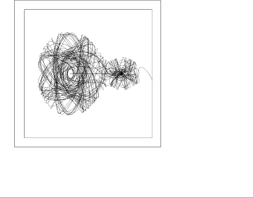
appear ﬁxed in position. Figure 2.1 shows a typical path of the asteroid. The hor-

izontal line segment in the center represents the (stationary) distance between

the two larger bodies: The large one is at the left end of the segment and the

medium one is at the right end. The tiny body moves back and forth between

the two larger bodies in a seemingly unpredictable manner for a long time. The

asteroid gains speed as it is ejected toward the right with sufﬁcient momentum so

Figure 2.1 A trajectory of a tiny mass in the three-body problem.

Two larger bodies are in circular motion around one another. This view is of a

rotating coordinate system in which the two larger bodies lie at the left and right

ends of the horizontal line segment. The tiny mass is eventually ejected toward the

right. Other trajectories starting close to one of the bodies can be forever trapped.

T WO-DIMENSIONAL M APS

that it never returns. Other pictures, with different initial conditions, could be

shown in which the asteroid remains forever close to one of the stars.

This three-body system is called the “planar restricted three-body problem”,

but we will refer to it as the three-body problem. Poincar

e’s method of analysis

was based on the fact that the motion of the small mass could be studied, in a

rather nonobvious manner, by studying the orbit of a plane map (a function from

⺢

to ⺢

). He discovered the crucial ideas of “stable and unstable manifolds”,

which are special curves in the plane (see Section 2.6 for deﬁnitions).

On the basis of his entry Poincar

e was declared the winner. However,

he did not fully understand the nature of the stable and unstable manifolds at

that time. These manifolds can cross each other, in so-called homoclinic points.

Poincar

e was confused by these points. Either he thought they didn’t exist or

he didn’t understand what happened when they did cross. This error made his

general conclusions about the nature of the trajectories totally wrong. His error

was detected after he had been declared the winner but before his entry was

published. He eventually realized that the existence of homoclinic points implied

that there was incredibly complicated motion near those points, behavior we now

call “chaotic”.

Poincar

e worked feverishly to revise his winning entry. The article “Sur les

equations de la dynamique et le probl

eme des trois corps” (on the equations of

dynamics and the three-body problem) was published in 1890. In this 270-page

work, Poincar

e established convincingly that due to the possibility of homoclinic

crossings, no general exact formula exists, beyond Newton’s differential equations

arising from (2.6) and (2.7), for making predictions of the positions of the three

bodies in the future.

Poincar

e succeeded by introducing qualitative methods into an area of

study that had long been dominated by highly reﬁned quantitative methods. The

quantitative methods essentially involved developing inﬁnite series expansions

for the positions and velocities of the gravitational bodies. These series expansions

were known to be problematic for representing near-collisions of the bodies.

Poincar

e was able to show through his geometric reasoning that these inﬁnite

series expansions could not converge in general.

One of Poincar

e’s most important innovations was a simpliﬁed way to look

at complicated continuous trajectories, such as those resulting from differential

equations. Instead of studying the entire trajectory, he found that much of the

important information was encoded in the points in which the trajectory passed

through a two-dimensional plane. The order of these intersection points deﬁnes

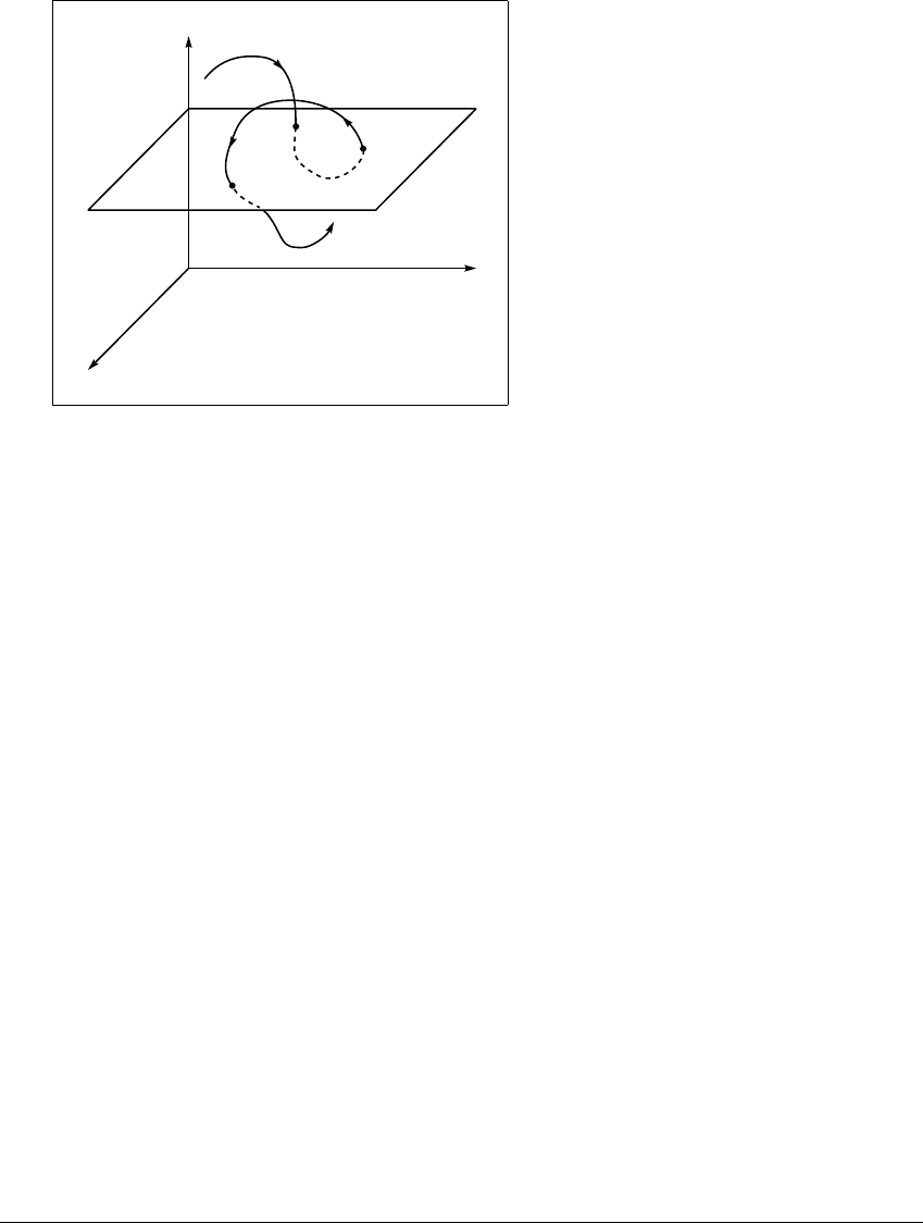
a plane map. Figure 2.2 shows a schematic view of a trajectory C. The plane S

is deﬁned by x

⫽ constant. Each time the trajectory C pierces S in a downward

2.1 MAT H E M AT IC A L M ODELS

Figure 2.2 A Poincar

e map derived from a differential equation.

The map G is deﬁned to encode the downward piercings of the plane S by the

solution curve C of the differential equation so that G(A) ⫽ B,andsoon.

direction, as at points A and B in Figure 2.2, we record the point of piercing

on the plane S. We can label these points by the coordinates (x

). Let A

represent the kth downward piercing of the plane and B the (k ⫹ 1)th downward

piercing. The Poincar

emapis the two-dimensional map G such that G(A) ⫽ B.

The Poincar

e map is similar in principle to the time-T map we considered above,

though different in detail. While the time-T map is stroboscopic (it logs the value

of a variable at equal time intervals), the Poincar

e map records plane piercings,

which need not be equally spaced in time. Although Figure 2.2 shows a plane,

more general surfaces can be used. The plane or surface is called a surface of

section.

Given A, the differential equations can be solved with A as an initial

value, and the solution followed until the next downward piercing at B.ThusA

uniquely determines B. This ensures that the map G is well-deﬁned. This map

can be iterated to ﬁnd all subsequent piercings of S. In general, the Poincar

map technique reduces a k-dimensional, continuous-time dynamical system to a

(k ⫺ 1)-dimensional map. Much of the dynamical behavior of the trajectory C is

present in the two-dimensional map G. For example, the trajectory C is periodic

(forms a closed curve, which repeats the same dynamics forever) if and only if the

plane map G has a periodic orbit.

Now we can explain how the differential equations of the three-body prob-

lem shown in Figure 2.1 led Poincar

e to a plane map. In our rotating coordinate

T WO-DIMENSIONAL M APS

system (where the two stars are ﬁxed at either end of the line segment) the dif-

ferential equations involve the position (x, y) and velocity (

y) of the asteroid.

These four numbers determine the current state of the asteroid.

There is a constant of the motion, called the Hamiltonian. For this problem

it is a function in the four variables that is constant with respect to time. It is

like total energy of the asteroid, which never changes. The following fact can be

shown regarding this Hamiltonian: for y ⫽ 0 and for any particular x and

x,the

Hamiltonian reduces to

⫽ C,whereC ⱖ 0. Thus when the vertical component

of the position of the asteroid satisﬁes y ⫽ 0, the vertical velocity component of

the asteroid is restricted to the two possible values ⫾



Because of this fact, it makes sense to consider the Poincar

e map, using up-

ward piercings of the surface of section y ⫽ 0. The variable y is the vertical com-

ponent of the position, so this corresponds to an upward crossing of the horizontal

line segment in Figure 2.1. There are two “branches” of the two-dimensional sur-

face y ⫽ 0, corresponding to the two possible values of

y mentioned above. (The

two dimensions correspond to independent choices of the numbers x and

x.) We

choose one branch, say the one that corresponds to the positive value of

y, for our

surface of section. What we actually do is follow the solution of the differential

equation, computing x, y,

y as we go, and at the instant when y goes from neg-

ative to positive, we check the current

y from the differential equation. If

y ⬎ 0,

then an upward crossing of the surface has occurred, and x,

x are recorded. This

deﬁnes a Poincar

e map.

Starting the system at a particular value of (x,

x), where y is zero and is

moving from negative to positive, signalled by

y ⬎ 0, we get the image F(x,

by recording the new (x,

x) the next time this occurs. The Poincar

emapF

is a two-dimensional map. What Poincar

e realized should now be clear to us.

Even this restricted version of the full three-body problem contains much of

the complicated behavior possible in two-dimensional maps, including chaotic

dynamics caused by homoclinic crossings, shown in Figure 2.24. Understanding

these complications will lead us to the study of stable and unstable manifolds, in

Section 2.6 at ﬁrst, and then in more detail in Chapter 10.

Work in the twentieth century has continued to reﬂect the philosophy

that much of the chaotic phenomena present in differential equations can be

approached, through reduction by time-T maps and Poincar

e maps, by studying

discrete-time dynamics. As you can gather from the three-body example, Poincar

maps are seldom simple to evaluate, even by computer. The French astronomer

M. H

enon showed in 1975 that much of the interesting phenomena present in

Poincar

e maps of differential equations can be found as well in a two-dimensional

2.1 MAT H E M AT IC A L M ODELS

quadratic map, which is much easier to simulate on a computer. The version of

enon’s map that we will study is

f(x, y) ⫽ (a ⫺ x

⫹ by, x). (2.8)

Note that the map has two inputs, x, y, and two outputs, the new x, y. The new

y is just the old x, but the new x is a nonlinear function of the old x and y.The

letters a and b represent parameters that are held ﬁxed as the map is iterated.

The nonlinear term x

in (2.8) is just about as unobtrusive as could be

achieved. H

enon’s remarkable discovery is that this “barely nonlinear” map dis-

plays an impressive breadth of complex phenomena. In its way, the H

enon map is

to two-dimensional dynamics what the logistic map G(x) ⫽ 4x(1 ⫺ x)istoone-

dimensional dynamics, and it continues to be a catalyst for deeper understanding

of nonlinear systems.

For now, set a ⫽ 1.28 and b ⫽⫺0.3. (Here we diverge from H

enon, whose

most famous example has b ⫽ 0. 3 instead.) If we start with the initial condition

(x, y) ⫽ (0, 0) and iterate this map, we ﬁnd that the orbit moves toward a period-

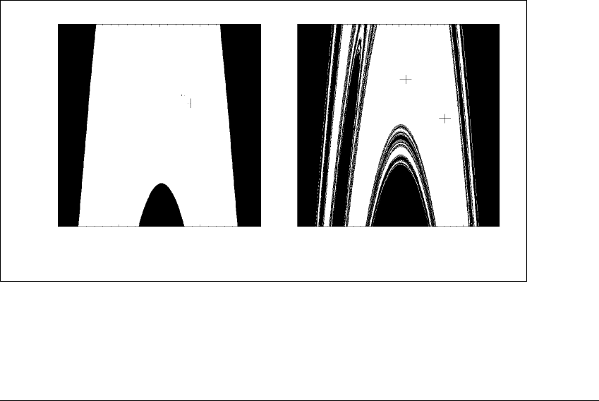
two sink. Figure 2.3(a) shows an analysis of the results of iteration with general

initial values. The picture was made by starting with a 700 ⫻ 700 grid of points

2.5

⫺2.5

⫺2.52.5

(a)

⫺2.52.5

(b)

Figure 2.3 A square of initial conditions for the H

enon map with

ⴝⴚ0

Initial values whose trajectories diverge to inﬁnity upon repeated iteration are

colored black. The crosses show the location of a period-two sink, which attracts

the white initial values. (a) For a ⫽ 1.28, the boundary of the basin is a smooth

curve. (b) For a ⫽ 1.4, the boundary is “fractal” .

T WO-DIMENSIONAL M APS

in [⫺2.5, 2.5] ⫻ [⫺2.5, 2.5] as initial values. The map (2.8) was iterated by

computer for each initial value until the orbit either converges to the period-two

sink, or diverges toward inﬁnity. Points in black represent initial conditions whose

orbits diverge to inﬁnity, and points in white represent initial values whose orbits

converge to the period-two orbit. The black points are said to belong to the basin

of inﬁnity, and the white points to the basin of the period-two sink. The boundary

of the basin consists of a smooth curve, which moves in and out of the rectangle

of initial values shown here.

✎ E XERCISE T2.1

Check that the period-two orbit of the H

enon map (2.8) with a ⫽ 1.28 and

b ⫽⫺0.3 is approximately 兵(0.7618, 0.5382), (0.5382, 0.7618)其. We will see

how to ﬁnd these points in Section 2.5.

➮ COMPUTER EXPERIMENT 2.1

Write a program to iterate the H

enon map (2.8). Set a ⫽ 1.28 and b ⫽⫺0.3

as in Figure 2.3(a). Using the initial condition (x, y) ⫽ (0, 0), create the period-

two orbit, and view it either by printing a list of numbers or by plotting (x, y)

points. Change a to 1.2 and repeat. How does the second orbit differ from the

ﬁrst? Find as accurately as possible the value of a between 1. 2and1.28 at which

the orbit behavior changes from the ﬁrst type to the second.

If we instead set a ⫽ 1.4, with b ⫽⫺0.3, and repeat the process, we see

quite a different picture. First, the points of the period-two sink have distanced

themselves a bit from one another. More interesting is that the boundary of the

basin is no longer a smooth curve, but is in a sense inﬁnitely complicated. This is

fractal structure, which we shall discuss in detail in Chapter 4.

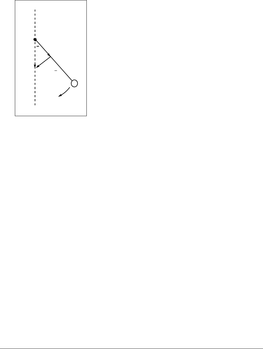
Next we want to show how a two-dimensional map can be derived from a

differential equations model of a pendulum. Figure 2.4 shows a pendulum swinging

under the inﬂuence of gravity. We will assume that the pendulum is free to swing

through 360 degrees. Denote by

␪

the angle of the pendulum with respect to the

vertical, so that

␪

⫽ 0 corresponds to straight down. Therefore

␪

and

␪

⫹ 2

␲

should be considered the same position of the pendulum.

2.1 MAT H E M AT IC A L M ODELS

mgsin

Figure 2.4 The pendulum under gravitational acceleration.

The force of gravity causes the pendulum bob to accelerate in a direction perpen-

dicular to the rod. Here

␪

denotes the angle of displacement from the downward

position.

We will use Newton’s law of motion F ⫽ ma to ﬁnd the pendulum equation.

The motion of the pendulum bob is constrained to be along a circle of radius l,

where l is the length of the pendulum rod. If

␪

is measured in radians, then the

component of acceleration tangent to the circle is l

␪

, because the component of

position tangent to the circle is l

␪

. The component of force along the direction

of motion is mg sin

␪

. It is a restoring force, meaning that it is directed in the

opposite direction from the displacement of the variable

␪

. We will denote the

ﬁrst and second time derivatives of

␪

(the angular velocity) and

␪

(the

angular acceleration) in what follows. The differential equation governing the

frictionless pendulum is therefore

␪

⫽ F ⫽⫺mg sin

␪

, (2.9)

according to Newton’s law of motion.

From this equation we see that the pendulum requires a two-dimensional

state space. Since the differential equation is second order, the two initial values

␪

(0) and

␪

(0) at time t ⫽ 0 are needed to specify the solution of the equation

after time t ⫽ 0. It is not enough to specify

␪

(0) alone. Knowing

␪

(0) ⫽ 0 means

that the pendulum is in the straight down conﬁguration at time t ⫽ 0, but we

can’t predict what will happen next without knowing the angular velocity at that

time. For example, if the angle

␪

is 0, so that the pendulum is hanging straight