Adlard E.R. (ed.) Chromatography in the Petroleum Industry
Подождите немного. Документ загружается.

2
Chapter
I
by means
of
valves. This complexity, which
is
more daunting in prospect than in
use, has led to a number of ready-configured chromatographic systems for many
of the application areas.
The thermal conductivity detector (TCD) and flame ionization detector (FID)
are the
two
most commonly used for hydrocarbon gases in the petroleum indus-
try.
Because many of the gases contain non-hydrocarbon components, the TCD,
as
a
universal detector,
is
essential. Its dynamic range allows it to be used also
for all the major and many of the minor components of most mixtures. The FID,
while the most commonly used detector in gas chromatography generally, can be
regarded as a specialist and specific detector
in
gas analysis. Process chroma-
tographs frequently use the TCD alone, to reduce the need for the extra facilities
needed
for
the use
of
the FID.
1.2
NATURAL
GAS
Hydrocarbon gases arise naturally from a variety
of
sources. Bacterial fermen-
tation under anaerobic conditions produces methane
or
marsh gas in great pro-
fusion, about 109 tonnes per year worldwide. Small accumulations
of
this type
of
gas can be found during tunnelling
or
other operations, and the same mecha-
nisms produce landfill gas from waste. Mine drainage gas is a methane-rich
mixture found where coal measures have been worked. However, the term natu-
ral gas is normally taken
to
refer to the fossil-based gaseous equivalent to oil and
coal, abstracted from ancient, large, deeply buried accumulations. This is the
sense in which the term is used in this chapter.
Natural gases can vary considerably in composition, from nearly pure nitrogen
to
nearly pure carbon dioxide to nearly pure methane. Fortunately for the indus-
try and the consumer, most natural gases consist mainly of methane, with small
amounts of inert gases (helium, nitrogen and carbon dioxide) and ethane and
higher alkanes in concentrations which diminish as their carbon number in-
creases.
By far the largest
use
of natural gas
is
as a fuel, where its accessibility via
wide-ranging distribution systems and its cleanness in terms of handling and
combustion products make it a popular choice for both domestic and industrial/
commercial markets. Other uses are as a chemical feedstock, as a source of pure
single hydrocarbon gases
or
(if present in sufficient quantities) of helium, and
as
a
moderator in nuclear reactors.
Current estimates indicate that the world has more reserves of natural gas than
of
oil at the present rate of consumption. Recent measures of worldwide produc-
tion give a figure of around
lo9
tonnes per year, which is comparable
to
the bac-
terial production referred to earlier.
The analysis
of
hydrocarbon gases
3
Natural gas is part of a continuum of hydrocarbons, ranging from methane to
the heaviest ends of oil, which are found in geological accumulations. Pressure
and temperature conditions in the reservoir are such that there is no distinction
between what we regard as gases and liquids; this only occurs when the fluid has
been extracted and is subject to conditions at which this discrimination is possi-
ble. Whether an accumulation is regarded as a gas or oil field is only a matter of
the relative proportions of the hydrocarbons. Natural gas fields always contain
liquids, usually in the form of a lightish condensate, and oil fields always contain
associated gases.
Gas separated from a natural gas field will burn in that form, but is usually
treated to remove or to control the levels of particular components, for opera-
tional, or contractual, or legislative reasons. Hydrogen sulphide, being toxic and
corrosive, is invariably subject to very low
(parts
per million) specification lim-
its,
and is typically removed in an amine plant. Carbon dioxide is
less
acidic,
but
still potentially corrosive at the pressures used for gas transmission, and its con-
centration is also controlled, usually to low percentage levels. It can be removed
by an alkali scrubbing process. Water is removed by glycol scrubbing, since the
presence of liquid water increases the corrosive effect of acid gases, and because
it can form solid methane hydrate, a clathrate compound, under certain pressure
and temperature conditions. Potential hydrocarbon liquids are also removed,
usually by chilling, sometimes by adsorption. This is to prevent their condensa-
tion downstream of the processing plant.
The fact that natural gas, once processed at the wellhead
or
reception termi-
nal, is in the form which virtually every consumer can accept without modifica-
tion has given rise to very complex and detailed pipeline systems, which cross
international boundaries and finally enter the consumer’s premises.
In
Western
Europe,
most
countries have access to pipeline supplies from Holland, the North
Sea, Siberia and Algeria in addition to their own indigenous sources. In the
United States, which is the home of long-distance natural gas transmission,
pipeline systems include Canada and Mexico as well as extensive offshore net-
works.
Properties and behaviour of natural gas have been reviewed by Melvin
[
13.
A
large number of papers on quality specifications, physical properties, sampling,
odorization and analysis of natural gas, and on calibration gases and standardi-
zation are collected in the proceedings of the
1986
Gas Quality Congress [2].
Analysis of natural gas is carried out for a range of purposes, and the choice
of analytical method is often dictated by the reason for the analysis being re-
quired. There are three basic purposes for analysis:
-
identification of source,
-
calculation of physical properties, and
-
measurement of specific minor components because of their particular
characteristics.
References
p.
40
4
Chapter
I
For identification of source, the concentrations of the inert components and
the ratios of a small number of hydrocarbons are good indicators; the analysis
need not be detailed. An example of specific minor component analysis is the
measurement
of
odorants; the analysis
is
clearly targeted upon
a
few compo-
nents, probably using a selective detector, and the composition of the main com-
ponents is without interest, except insofar as they may interfere with the meas-
urement. Calculation of properties
is
the most common need for analysis, with
calorific value the most usual target.
The following is a list of some of the properties of natural gas which are cal-
culable from analysis. It is not comprehensive, but describes those most fre-
quently used. Most properties can be measured directly, but independently of
each other; a properly configured analytical method allows calculation of all.
1.
Culorijic value
(CV):
Natural gas
is
bought and sold in units of volume, as
a
source of energy, hence the importance of
CV
as energy per unit of volume.
2.
Relative
density
(RD):
This is the density of a gas relative
to
dry air
(=
1.000).
It
is used in metering calculations and for the Wobbe index (see be-
low).
3.
Wobbe index
(WI):
Gases from different sources must be assessed for their
inter-changeability, which represents the effectiveness with which a gas of com-
position
B
will burn on an appliance designed for a gas of composition
A.
WI
is
an empirical measure of the ability to supply heat to
a
burner, and is the most
important characteristic in determining interchangeability. It
is
calculated by di-
viding the CV by the square root of the
RD.
4.
Compression factor
(Z):
Compression factor appears in the modified ideal
gas equation
PV=
nZRT,
and arises from gas phase interactions. For hydro-
carbon gases and their mixtures over normal temperature and pressure ranges,
Z
is
always less than
1,
which means that a defined volume of gas at a defined
pressure
will
contain more moles than predicted from ideal behaviour by a factor
of
1/Z.
At ambient conditions,
Z
for most natural gases is around 0.997, but the
correction is much more significant at higher pressures. At 70 bar, typical of
transmission pressures,
Z
is usually less than 0.9. Metering at high pressure is
therefore very dependent upon accurate measurement or calculation of
Z.
5.
Hydrocarbon dewpoint:
Retrograde condensation is the phenomenon
whereby a liquid phase can separate from a hydrocarbon gas mixture
as
it is de-
pressurized at a constant temperature. It is another feature of gas phase interac-
tions, and may be regarded as a form of “gas phase solubility”, with components
coming out of solution as the pressure binding the molecules together is re-
leased.
6.
.Joule-Thomson coefficient:
This property influences the extent of cooling
as
a
gas is expanded.
As
the pressure of natural gas
is
reduced, the amount of
pre-heating necessary to avoid hydrocarbon condensation can be calculated.
The analysis
of
hydrocarbon gases
5
1.2.1
Analytical requirements
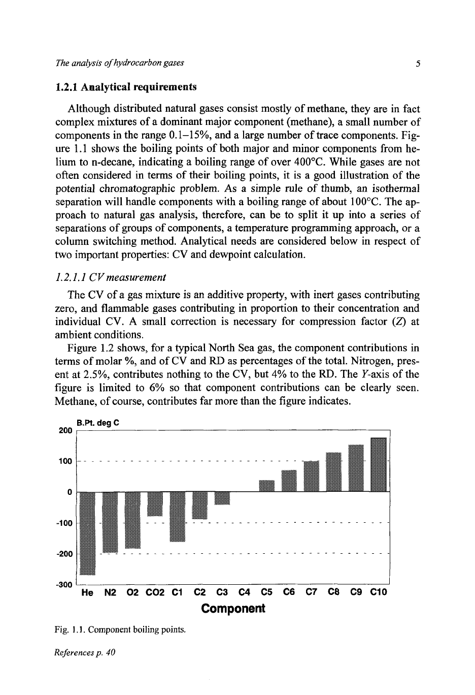
Although distributed natural gases consist mostly of methane, they are in fact
complex mixtures of a dominant major component (methane), a small number
of
components in the range
0.1-15%,
and a large number of trace components. Fig-
ure 1.1 shows the boiling points of both major and minor components from he-
lium to n-decane, indicating a boiling range of over
400°C.
While gases are not
often considered in terms of their boiling points, it is a good illustration
of
the
potential chromatographic problem.
As
a simple rule
of
thumb, an isothermal
separation will handle components with a boiling range of about
100°C.
The ap-
proach
to
natural gas analysis, therefore, can be to split it up into a series
of
separations
of
groups
of
components, a temperature programming approach,
or
a
column switching method. Analytical needs are considered below in respect of
two
important properties:
CV
and dewpoint calculation.
1.2.1.1
CVmeasurement
The
CV
of
a gas mixture is an additive property, with inert gases contributing
zero, and flammable gases contributing in proportion to their concentration and
individual
CV.
A
small correction is necessary for compression factor
(2)
at
ambient conditions.
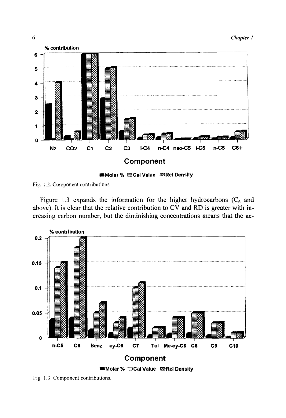
Figure
1.2
shows, for a typical North Sea gas, the component contributions in
terms of molar
%,
and of
CV
and
RD
as percentages
of
the total. Nitrogen, pres-
ent at
2.5%,
contributes nothing to the
CV,
but
4%
to the
RD.
The Y-axis of the
figure
is
limited to
6%
so
that component contributions can be clearly seen.
Methane, of course, contributes far more than the figure indicates.
B.R.
deg
C
200
I
I
-300
I
1
He N2 02 C02 C1 C2 C3 C4 C5 C6 C7 C8 C9 C10
Component
Fig.
1.
I.
Component boiling points.
References
p.
40
6
%
Contribution
Chapter
I
N2
C02
C1
C2
C3
164
nC4
nee=
IC5
n-C5
C6+
Component
IMoiar
%
BCal Value =Re1 Density
Fig.
1.2.
Component contributions.
Figure
1.3
expands the information
for
the higher hydrocarbons
(C,
and
above). It
is
clear that the relative contribution to
CV
and
RD
is
greater with in-
creasing carbon number, but the diminishing concentrations means that the ac-
0.2
0.15
0.1
0.05
0
%
contribution
17
nC5
C6
Benr cyC6
C7
To1
MecyC6
CB
C9
C10
Component
mMolar
%
BCal
Value
BRel
Denslty
Fig.
1.3.
Component contributions.
The analysis ofhydrocarbon gases
7
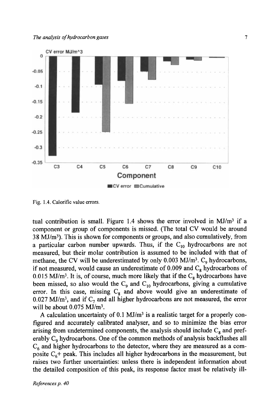
Fig.
1.4.
Calorific value errors.
tual contribution is small. Figure
1.4
shows the error involved in MJ/m3 if a
component or group of components is missed. (The total CV would be around
38
MJ/m3). This is shown for components or groups, and also cumulatively, from
a particular carbon number upwards. Thus,
if
the Clo hydrocarbons are not
measured, but their molar contribution is assumed to be included with that of
methane, the CV will be underestimated by only
0.003
MJ/m3. C, hydrocarbons,
if not measured, would cause an underestimate of
0.009
and
C,
hydrocarbons of
0.015
MJ/m3. It is, of course, much more likely that if the C, hydrocarbons have
been missed,
so
also would the
C,
and
C,,
hydrocarbons, giving a cumulative
error. In this case, missing C, and above would give an underestimate of
0.027
MJ/m3, and if C, and all higher hydrocarbons are not measured, the error
will be about 0.075 MJ/m3.
A
calculation uncertainty of
0.1
MJ/m3 is a realistic target for a properly con-
figured and accurately calibrated analyser, and
so
to
minimize the bias error
arising from undetermined components, the analysis should include
C,
and pref-
erably C, hydrocarbons. One of the common methods of analysis backflushes all
C,
and higher hydrocarbons to the detector, where they are measured as a com-
posite
C,+
peak. This includes all higher hydrocarbons in the measurement, but
raises
two
further uncertainties: unless there is independent information about
the detailed composition of this peak, its response factor must be relatively ill-
References
p.
40
x
Chapter
1
defined, and
so
must its contribution to CV
or
other properties. In fact, the CV of
the
C,+
fraction of many gases can be approximated by that of n-hexane without
significant error. Components such
as
benzene and toluene, and to
a
lesser extent
the cyclo-alkanes have lower CVs than alkanes of equivalent carbon number,
and if present in reasonable proportion can counteract the higher CV contribu-
tions
of
C, and higher alkanes.
1.2.
I
2
lfydrocarbon
dewpoint
calculation
Calculation of hydrocarbon dewpoint temperature is complex, as interactions
between components must be accounted for in addition to individual component
properties, Higher hydrocarbons make a considerable contribution, because of
their relatively low vapour pressures.
For
CV
calculation, it is normal to
con-
sider all alkanes of a particular carbon number as a group. Since the CVs of
al-
kane isomers are very similar, this is realistic and involves virtually no
loss
of
accuracy. The same approach is incorrect for hydrocarbon dewpoint calculation,
as
the contributions of isomers differ. This creates
two
problems: computer
packages for these calculations cannot handle as many components as a detailed
analysis can measure, and even the most detailed analysis cannot definitely
identify all the peaks which it separates, nor find the appropriate properties
for
those components through
a
database.
A
typical computer program will handle
30
components, and one approach
has been to group alkane isomers as if their sum was represented by the n-alkane
of that carbon number. Since the n-alkane has the highest boiling point of the
series, this approach will over-estimate the contributions to dewpoint tempera-
ture, and
so
has the advantage of a built-in safety margin.
A
more accurate ap-
proach
is
to input data for groups of components as that of fractions rather than
components, assuming that the program allows components and fractions to be
mixed.
Detailed separation of higher hydrocarbons is most likely to be on the basis of
boiling point, as in simulated distillation. Each peak in the chromatogram, with-
out being identified, can have a boiling point allocated to it based upon its reten-
tion time relative to bracketing n-alkanes, a carbon number based upon its posi-
tion in the chromatogram, and hence an
FID
response factor and molar percent-
age. It
is
therefore practicable to consider a group
of
hydrocarbons, such as the
C,
alkanes, not as n-C, but as the C, fraction. This fraction has
a
defined molecu-
lar weight and density, a molar concentration and a calculated average boiling
point. This
is
sufficient information to be able to input the
C,
data as a fraction
with properties which more realistically represent its contribution. The same ap-
proach can
be
used
for
C,, C,, C,, and any higher hydrocarbon groups which
may be measured.
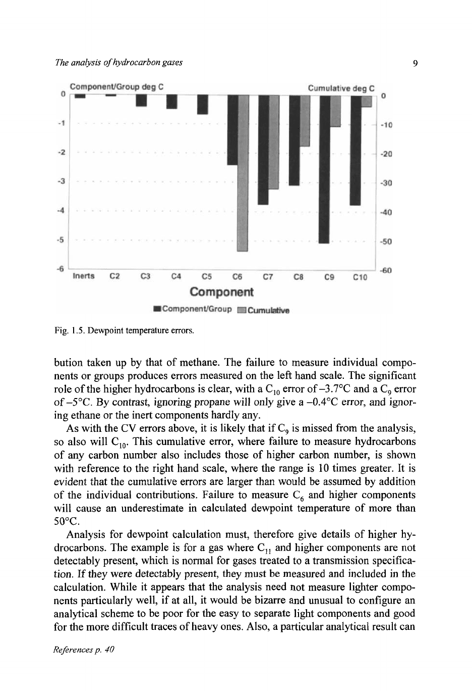
Figure
1.5
shows the errors involved in dewpoint temperature calculation if
components or groups of components are not measured, and their molar contri-
The analysis
of
hydrocarbon gases
9
Fig.
1.5.
Dewpoint temperature errors.
bution taken up by that of methane. The failure to measure individual compo-
nents or groups produces errors measured on the left hand scale. The significant
role of the higher hydrocarbons is clear, with a
C,,
error of
-3.7"C
and a
C,
error
of
-5°C.
By contrast, ignoring propane will only give a
-0.4"C
error, and ignor-
ing ethane or the inert components hardly any.
As
with the
CV
errors above, it is likely that if
C,
is
missed from the analysis,
so
also will
Clo.
This cumulative error, where failure to measure hydrocarbons
of any carbon number also includes those of higher carbon number, is shown
with reference to the right hand scale, where the range is 10 times greater. It is
evident that the cumulative errors are larger than would be assumed by addition
of the individual contributions. Failure to measure
C,
and higher components
will cause an underestimate in calculated dewpoint temperature of more than
50°C.
Analysis for dewpoint calculation must, therefore give details of higher hy-
drocarbons. The example
is
for a gas where
C,,
and higher components are not
detectably present, which
is
normal for gases treated to a transmission specifica-
tion.
If
they were detectably present, they must be measured and included in the
calculation. While it appears that the analysis need not measure lighter compo-
nents particularly well, if at all, it would be bizarre and unusual to configure an
analytical scheme to be poor for the easy to separate light components and good
for the more difficult traces of heavy ones. Also, a particular analytical result can
References
p.
40
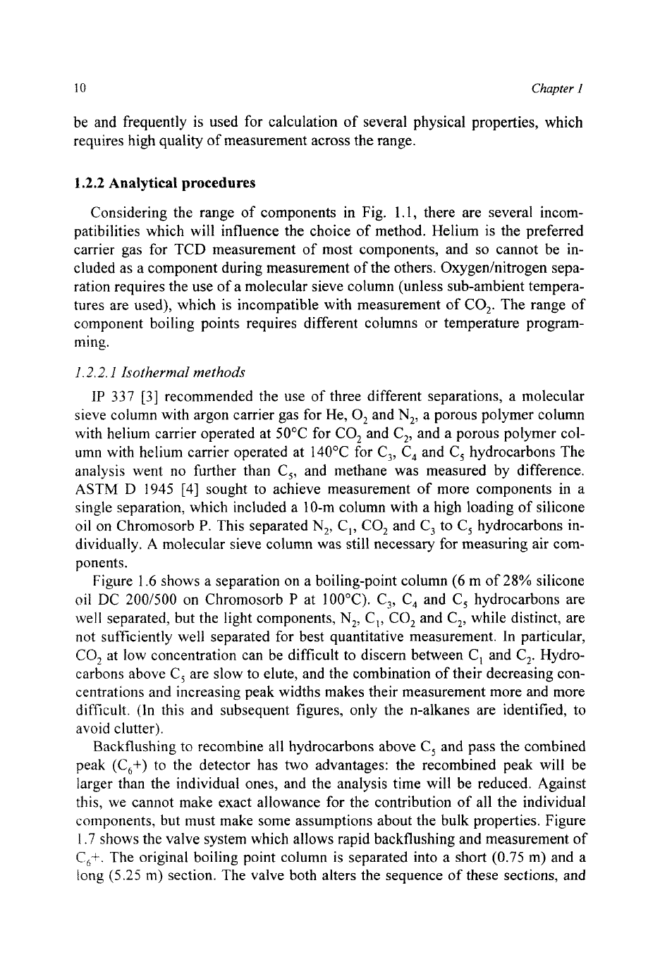
10
Chapter
I
be and frequently
is
used for calculation of several physical properties, which
requires high quality of measurement across the range.
1.2.2
Analytical
procedures
Considering the range of components in Fig.
1.1,
there are several incom-
patibilities which will influence the choice of method. Helium is the preferred
carrier gas
for
TCD measurement of most components, and
so
cannot be in-
cluded as a component during measurement of the others. Oxygednitrogen sepa-
ration requires the use of a molecular sieve column (unless sub-ambient tempera-
tures are used), which
is
incompatible with measurement
of
CO,. The range
of
component boiling points requires different columns
or
temperature program-
ming.
1.2.2.
I
Isothermal
methods
IP 337 [3] recommended the use
of
three different separations,
a
molecular
sieve column with argon carrier gas for He,
0,
and
N,,
a porous polymer column
with helium carrier operated at 50°C for CO, and
C,,
and a porous polymer col-
umn with helium carrier operated at
140°C
for C,, C, and C, hydrocarbons The
analysis went no further than
C,,
and methane was measured by difference.
ASTM
D
1945 [4]
sought to achieve measurement
of
more components in a
single separation, which included a 10-m column with a high loading
of
silicone
oil on Chromosorb
P.
This separated
N,,
C,,
CO, and C, to
C,
hydrocarbons in-
dividually.
A
molecular sieve column was still necessary for measuring air com-
ponents.
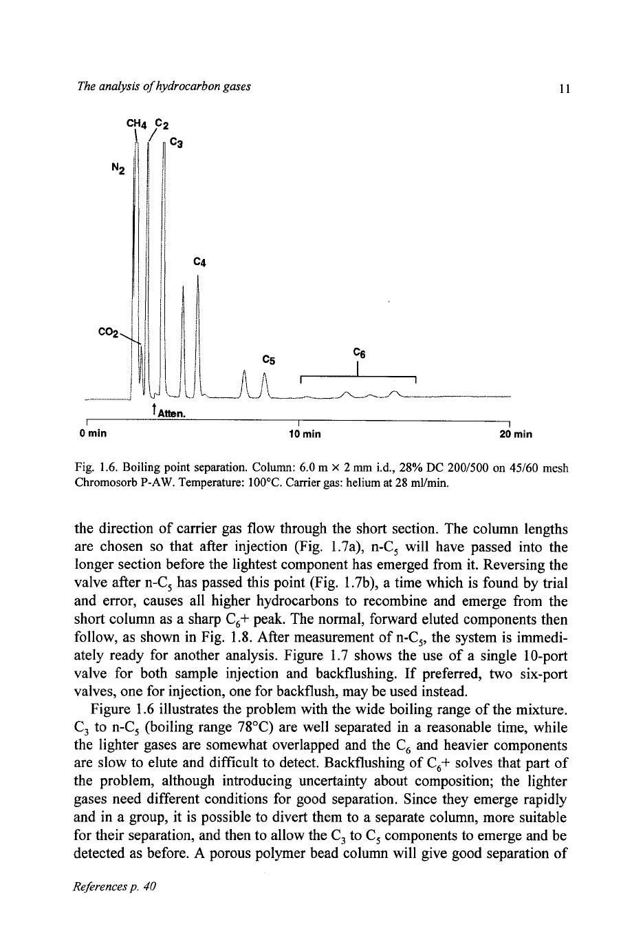
Figure
1.6
shows
a
separation
on
a boiling-point column
(6
m of
28%
silicone
oil
DC
200/500
on Chromosorb
P
at 100°C).
C,,
C,
and
C,
hydrocarbons are
well separated, but the light components,
N,,
C,, CO, and C,, while distinct, are
not sufficiently well separated for best quantitative measurement. In particular,
CO,
at
low
concentration can be difficult
to
discern between
C,
and C,. Hydro-
carbons above
C,
are slow
to
elute, and the combination of their decreasing con-
centrations and increasing peak widths makes their measurement more and more
difficult. (In this and subsequent figures, only the n-alkanes are identified, to
avoid clutter).
Backflushing to recombine all hydrocarbons above C, and pass the combined
peak
(C,+)
to the detector has
two
advantages: the recombined peak will be
larger than the individual ones, and the analysis time will be reduced. Against
this, we cannot make exact allowance for the contribution of all the individual
components, but must make some assumptions about the bulk properties. Figure
1.7 shows the valve system which allows rapid backflushing and measurement of
C,i.
The original boiling point column
is
separated into a short
(0.75
m) and a
long
(5.25
m) section. The valve both alters the sequence
of
these sections, and
The analysis
of
hydrocarbon gases
11
fAlten.
I
I
I
0
min
10
min
20
min
Fig.
1.6.
Boiling point separation. Column:
6.0
m
X
2
mm id.,
28%
DC
200/500
on
45/60
mesh
Chromosorb
P-AW.
Temperature:
100°C.
Carrier gas: helium at
28
ml/min.
the direction of carrier gas flow through the short section. The column lengths
are chosen
so
that after injection (Fig. 1.7a), n-C, will have passed into the
longer section before the lightest component has emerged from it. Reversing the
valve after n-C, has passed this point (Fig. 1.7b), a time which is found by trial
and error, causes all higher hydrocarbons to recombine and emerge from the
short column as a sharp C,+ peak. The normal, forward eluted components then
follow, as shown in Fig.
1.8.
After measurement of n-C,, the system is immedi-
ately ready for another analysis. Figure 1.7 shows the use of a single 10-port
valve for both sample injection and backflushing. If preferred,
two
six-port
valves, one for injection, one for backflush, may be used instead.
Figure
1.6
illustrates the problem with the wide boiling range of the mixture.
C, to n-C, (boiling range 78°C) are well separated in a reasonable time, while
the lighter gases are somewhat overlapped and the C, and heavier components
are slow to elute and difficult to detect. Backflushing of C,+ solves that part of
the problem, although introducing uncertainty about composition; the lighter
gases need different conditions for good separation. Since they emerge rapidly
and in a group, it is possible to divert them to a separate column, more suitable
for their separation, and then to allow the C, to C, components to emerge and be
detected as before. A porous polymer bead column will give good separation of
References
p.
40