Zdunkowski W., Trautmann T., Bott A. Radiation in the atmosphere: A course in Theoretical Meteorology

Подождите немного. Документ загружается.

11.2 Remote sensing based on short- and long-wave radiation 415

when z increases from z = 0toz = z

. From the ﬁgure it will be seen that at a

particular altitude z = z

the weighting function exhibits a maximum. Obviously,

with increasing absorption the location of the maximum z

moves upward. This can

be explained by the fact that for a strongly absorbing gas T

(z, z

) already vanishes

at high altitudes. With decreasing absorption z

moves downward correspondingly.

Let us consider the idealized situation where the weighting function is a δ-

function, i.e.

(z, z

) = δ(z − z

) (11.24)

Inserting this equation into (11.21) leads to

+,ν

) = I

+,ν

(0)T

(0, z

) + B

) (11.25)

Hence, in addition to the contribution coming from the lower boundary, the satellite

instrument detects radiation coming directly from the level z

. If similar weight-

ing functions exist for other wavelengths λ

and if the corresponding weighting

functions W

have their delta function peaks at z

m,i

, then this idealized situation

directly provides the atmospheric temperature proﬁle at the discrete set of altitudes

m,i

Unfortunately, atmospheric weighting functions always possess a ﬁnite width,

and in most cases these weighting functions computed for different wave numbers

overlap substantially. Therefore, the inversion of the temperature proﬁle from a set

of nadir radiance measurements is a complicated and difﬁcult task.

In the atmospheric window region we have

≈ 1,

≈ 0 (11.26)

Inserting this equation into (11.21) we obtain

+,ν

) ≈ I

+,ν

(0) (11.27)

i.e. for most practical purposes the instrument registers the signal emitted by the

ground. If the emissivity of the ground is equal to 1 it follows from (11.20) that

+,ν

) = B

) (11.28)

Thus the instrument aboard a satellite measures the black body emission of the

Earth’s surface. This means that the temperature T

of the ground can be determined

by inverting (11.28).

If the observation takes place in a strong absorption band, then the absorption

coefﬁcient can be assumed to be large so that

(0, z

) ≈ 0 (11.29)

416 Remote sensing applications of radiative transfer

This statement implies that any ground contribution to the radiation ﬁeld at the

satellite’s position can be safely neglected. Now (11.21) reduces to

+,ν

) =



(z)

(z, z

)dz (11.30)

This formula has important applications. For an absorber gas with constant mixing

ratio, such as carbon dioxide in the 4.3 and 15

µm bands, or oxygen in the 5 mm

microwave band (i.e. the so-called 60 GHz O

complex), the weighting function

can be computed very easily, that is the signal observed by the instrument aboard

the satellite can be exploited to invert the vertical temperature proﬁle. This makes

it necessary to select a speciﬁc set of wavelengths so that for each wavelength the

weighting function attains its maximum contribution to the observed signal at a

particular altitude range.

Note that the determination of the temperature proﬁle heavily relies on the

assumption that the mixing ratio of the considered trace gas is constant with height.

Otherwise both the concentration proﬁle as well as the temperature proﬁle would

be unknown quantities making the inversion much more difﬁcult.

Clouds pose a peculiar problem in atmospheric remote sensing because in the

visible and long-wave spectral wavelength region they are not transparent. As a con-

sequence, atmospheric parameters can only be retrieved for the altitude range above

the cloud top. However, it becomes possible to invert the cloud top temperature.

So far we have considered only the nadir viewing geometry. However, the pre-

vious discussion can be generalized to abritrary viewing directions using scanning

instruments. As seen from the satellite’s orbit such instruments provide a larger

areal coverage as compared to instruments which mainly look in nadir direction.

(2) Ground-based observations

In the case of ground-based observations of the long-wave sky radiation we assume

an isotropic radiation ﬁeld. Utilizing the boundary conditions (11.20) the downward

radiance at ground level expressed in z coordinates follows from (2.122)

−,ν

(0,µ) =−



(z)

(0, z,µ)dz =−



(z)W

(0, z,µ)dz (11.31)

with

(0, z,µ) = exp



−



abs,ν



)dz



(11.32)

and where µ is the direction of observation. A similar analysis as in the case

of spaceborne observations leads to the following conclusions for ground-based

observations: The weighting function typically decreases strongly with increasing

altitude. Therefore, the main contributions to the detected signal originate from the

11.3 Inversion of the temperature proﬁle 417

lower troposphere thus limiting information extraction to the lowermost parts of

the atmosphere. This type of observation geometry in the long-wave spectral region

is of much less importance than radiance measurements from satellites. The only

exception is the observation of signals in close proximity to the ﬂanks of the strong

absorption bands of atmospheric trace gases leading to a complete sounding of the

atmosphere from ground level to higher altitudes.

11.3 Inversion of the temperature proﬁle

Using a radiometer in the long-wave electromagnetic spectrum aboard a satellite,

one can measure the upwelling radiance in several spectral regions that are called

channels. As discussed previously, the information content within an absorption

band of a speciﬁc trace gas can be exploited to retrieve the atmospheric temperature

proﬁle. We will now show how to proceed.

Let us start with the radiative transfer equation of the infrared spectrum, cf.

(2.113)

dτ

(τ,µ) = I

(τ,µ) − B

(τ ) (11.33)

The monochromatic differential optical depth is given by

dτ = k

du with du =−ρ

abs

(z)dz (11.34)

where k

is the spectral absorption coefﬁcient, u is the absorber amount and ρ

abs

the density of the absorber gas. Employing the hydrostatic equation we can relate

optical depth changes to changes in total atmospheric pressure

dτ = k

abs

dp with q

abs

(11.35)

Here q

abs

is the mass concentration of the trace gas and ρ is the air density. Substi-

tuting (11.35) into (11.33) we obtain for the change in radiance

(p,µ) =

[

(p,µ) − B

(p)

]

abs

dp (11.36)

For a nadir-looking instrument radiation is observed within a small solid angle

element centered around µ = 1 and the monochromatic transmission between the

top of the atmosphere and the pressure level p is given by

(p) = exp



−





abs



)dp



(11.37)

418 Remote sensing applications of radiative transfer

In this case the solution to (11.33) can be written as

(0) = I

(τ

) exp(−τ

) +



(τ



) exp(−τ



)dτ



(11.38)

where τ

is the total optical depth at z = 0 corresponding to the surface pressure p

Assuming that at τ

the surface radiates like a black body with temperature T ( p

)

and using the relation

∂T

∂p

dp =−T

dτ (11.39)

we can write the upwelling radiance for µ = 1 at the top of the atmosphere as

(0) = B

) +



(p)

∂T

∂p

dp (11.40)

Recall that ∂T

(p)/∂ p is the weighting function which multiplies the Planck func-

tion for the upwelling radiation emanating from an elementary atmospheric layer

of thickness dp.

Equation (11.40) is valid for monochromatic radiation only. In practice, however,

a radiation instrument is only capable of detecting radiation within a ﬁnite spectral

band (ν

,ν

) with central frequency ¯ν. The width of the interval and the sensitivity

of the radiometer are characterized by the response function φ

. Thus the radiation

detected by the radiometer may be expressed by

¯ν

(0) =



(0)dν



dν



dν





)dν +



(p)

∂T

∂p

dp dν



(11.41)

The mean transmission is deﬁned as

¯ν

(p) =



(p)dν



dν

(11.42)

so that the average weighting function is given by

∂T

¯ν

∂p



∂T

∂p

dν



dν

(11.43)

Note that the average weighting function now contains the sensitivity or the efﬁ-

ciency of the instrument. We may apply the approximation that within the given

frequency interval the Planck function varies linearly with respect to ν permitting

11.3 Inversion of the temperature proﬁle 419

us to replace B

by its mean value B

¯ν

. In this case B

¯ν

can be extracted from the

frequency integral. Inserting then (11.42) and (11.43) into (11.41) yields

¯ν

(0) = B

¯ν

) +



¯ν

(p)

∂T

¯ν

∂p

(11.44)

where we have also assumed that the frequency integral over the response function

is independent of pressure p.

The fundamental principle for deriving the temperature proﬁle of the atmosphere

from infrared soundings using satellite instruments is based on (11.44). This is due

to the fact that the Planck function contains the temperature information, while the

transmission of the atmosphere is associated with the absorption coefﬁcient and

the vertical proﬁle of the trace gas under consideration. Thus the observed radiation

must contain information on the proﬁles of both the atmospheric temperature as

well as the trace gas concentration.

As a particular example let us consider the infrared atmospheric window region

where, except for the 9.6

µm ozone band, absorption effects of atmospheric gases

are relatively insigniﬁcant. Therefore, observations of the upwelling radiance at the

top of the atmosphere in the atmospheric window are practically directly related to

the Planck radiation emitted by the surface, i.e.

¯ν

(0) ≈ B

¯ν

) (11.45)

has its main absorption band in the wavelength region stretching from 12–18

µm. With the exception of small-scale local effects, for instance due to biomass

burning and other anthropogenic effects, the mixing ratio of CO

is essentially

constant vertically and horizontally. Presently we may use

≈ 5.47 × 10

−4

(11.46)

being equivalent to a volume mixing ratio of 360 ppmv. The line intensities, the

position of all spectral lines and the line half-widths for CO

are known with high

precision from laboratory or theoretical results. Thus the spectral transmission

function and the weighting function for CO

can be calculated very accurately as a

function of pressure and temperature using model distributions. In many cases the

uncertainties in T and p are not essential.

Once a temperature proﬁle has been found by inverting the B

¯ν

functions using

suitable model values of T and p, we may repeat the transmission function calcula-

tions by employing the inverted temperature proﬁle and repeating the calculations

to obtain a new temperature proﬁle. We will soon return to this problem.

Given the surface temperature T ( p

) by inversion of (11.45), the vertical temper-

ature proﬁle T ( p ) can be found by inverting (11.44) for a set of channels in the CO

420 Remote sensing applications of radiative transfer

absorption band. Based on the temperature retrieval using CO

, nadir observation

in spectral absorption bands of various other trace gases, such as O

O and CH

could then be employed to derive total column contents or even proﬁle information

for these trace gases. In the following we will limit the discussion to the derivation

of the temperature proﬁle based on CO

In the CO

absorption band there exist several regions where the transmission

function approaches zero, so that the thermal signal emitted by the surface does not

reach the top of the atmosphere, i.e.

¯ν

) ≈ 0 (11.47)

Then (11.44) simpliﬁes to

¯ν

(0) ≈



¯ν

(p)

∂T

¯ν

∂p

dp (11.48)

For a set of different frequency bands the transmission and weighting functions

have to be computed as functions of pressure and temperature. Due to the frequency

dependence of the Planck function the average B

¯ν

will change from one frequency

band to the other. Therefore, it is necessary to eliminate the frequency dependence

in (11.48).

Within the CO

15 µm band the Planck function can be expressed as a linear

function

¯ν

(p) = α

¯ν

(p) + β

¯ν

(11.49)

where ν

is a ﬁxed reference frequency close to the center of the 15 µm band, and

¯ν

and β

¯ν

are ﬁt constants. Using this linear expression for the Planck function in

(11.48) leads to

¯ν

(0) − β

¯ν



¯ν

(p)

∂T

¯ν

∂p

dp (11.50)

It is customary to introduce the new functions

g(¯ν) =

¯ν

(0) − β

¯ν

, f (p) = B

¯ν

(p), K(¯ν, p) =

∂T

¯ν

∂p

(11.51)

Then (11.50) can be reformulated as

g(¯ν) =



f ( p)K(¯ν, p)dp (11.52)

This is a Fredholm integral equation of the ﬁrst kind. The weighting function

K(¯ν, p) is the so-called kernel of the integral equation. f ( p) is the function to be

11.3 Inversion of the temperature proﬁle 421

determined by employing a set of measurements g(¯ν

), i = 1,...,M, where M is

the total number of channels provided by the infrared radiometer.

In a ﬁrst step we will discuss the kernel K of the integral equation. The spectrally

averaged transmission function can be written as

¯ν

(p) =

ν



ν

exp



−





)dp



dν (11.53)

with ν = ν

− ν

. For illustrative purposes we have assumed an ideal instrument,

i.e. φ

= 1. For altitudes below about 30–40 km Lorentz broadening dominates

spectral line broadening so that simultaneous Doppler broadening can be safely

neglected. Inserting the absorption coefﬁcient for the Lorentz line shape, see (7.15),

and neglecting the temperature dependence of the Lorentz half-width so that

(p, T ) = α

L,0

≈ α

L,0

(11.54)

we obtain for the transmission the expression

¯ν

(p) =

ν



ν

exp



−





i=1

[T ( p



)]

L,i



)

(ν − ν

0,i

)

+ α

L,i



)





dν

(11.55)

where we summed over a total of L individual Lorentz lines contained in the spectral

interval ν.

In principle, the full temperature dependence of the absorption coefﬁcient has to

be taken into account. A particular problem for setting up the inversion of (11.44) is

that a priori we do not even know a rough approximation of the temperature proﬁle

that is needed to get the iteration started. As an initial guess one, therefore, assumes

a temperature proﬁle which is climatologically representative for the actual position

of the satellite.

Wark and Fleming (1966) computed for the US standard atmosphere the kernel

function K for six different rather narrow wave number bands ¯ν

, i = 1,...,M = 6

located within the 15

µmCO

band. Figure 11.10 depicts the vertical variation of

∂T

¯ν

(p)/ log p versus log p.

To make the inversion of (11.44) possible, the individual kernel functions

(p) = K(¯ν

, p) must possess distinct maxima in different altitude regions. If

this is the case for the selected narrow frequency bands, we may extract sufﬁ-

cient information from the upwelling radiation at the instruments level to con-

struct the desired vertical atmospheric proﬁle. As follows from inspection of Figure

11.10, the individual weighting functions overlap considerably which complicates

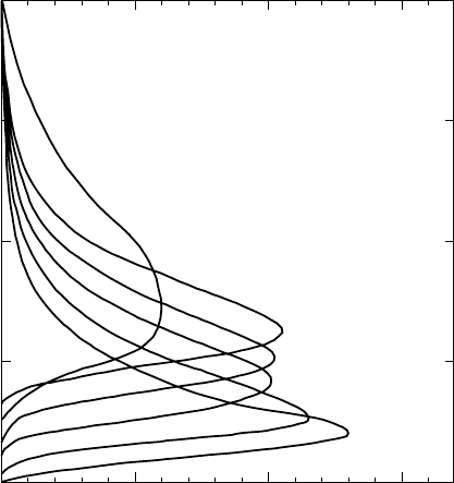
422 Remote sensing applications of radiative transfer

A : 669 cm

−1

B : 677.5cm

−1

C : 691cm

−1

D : 697cm

−1

E : 703cm

−1

F : 709 cm

−1

0.1

100

1000

0.0 0.5 1.0 1.5

∂τ/∂( log p)

p ( hPa)

Fig. 11.10 Weighting functions ∂T

¯ν

/∂p versus log p for six reference wave num-

bers applied to the 15 µmCO

band. (Redrawn from Wark and Fleming (1996),

with permission from the American Meteorological Society.)

the inversion process. The entire inversion is based on the set of observations

= g(¯ν

), i = 1,...,M which provide the necessary input information. Owing

to the overlapping kernel functions, we have to invert a system of N linear equations

for the unknown functions f ( p

), j = 1,...,N where N denotes the total number

of pressure levels. In case that the K

do not overlap, we would end up with N

independent equations which can be inverted directly. Since this is generally not

the case, it is advantageous to employ matrix methods to ﬁnd the proper solution.

11.3.1 Direct linear inversion

Employing the M radiance observations the mathematical problem is stated by a

set of M integral equations



f ( p)K

(p)dp, i = 1,...,M (11.56)

Usually the unknown function f ( p) can be expanded in terms of known represen-

tation functions W

(p), j = 1,...,N , which may involve Legendre polynomials

11.3 Inversion of the temperature proﬁle 423

or trigonometric functions so that

f ( p) =



j=1

(p) = B

¯ν

(p) (11.57)

The f

appearing in this equation are the unknown expansion coefﬁcients. For

(11.56) this leads to



j=1



(p)K

(p)dp, i = 1,...,M (11.58)

It is now convenient to introduce a M × N matrix A whose elements A

are given



(p)K

(p)dp (11.59)

leading to the compact notation



j=1

, i = 1,...,M (11.60)

In vector notation we ﬁnd

g = Af, g =













, f =













(11.61)

For the simple case where A is a square matrix with a nonvanishing determinant,

the solution to (11.61) is

f = A

−1

g (11.62)

Having found f we can compute the Planck function from (11.57) to ﬁnd the tem-

perature proﬁle T ( p).

Usually for a remote sensing problem the above assumption of an equal number

of unknowns and observations is not fulﬁlled so that the matrix A does not possess

an inverse A

−1

. In most cases the problem is underdetermined (M < N ) so that

we have more unknowns than independent observations. Thus the problem is ill-

posed. Even if A is a square matrix, the inverse A

−1

may still not exist if the

determinant of A is close to zero. This type of instability may arise for various

reasons such as (i) errors in the computation of the matrix elements A

, (ii) errors

when approximating the Planck function, (iii) round-off errors, or (iv) instrument

424 Remote sensing applications of radiative transfer

noise leading to observed radiances which involve random errors. In the Appendix

to this chapter we will give an illustrative example of an ill-posed problem.

11.3.2 Linear inversion with constraints

Consider the ill-posed problem



j=1

, i = 1,...,M (11.63)

Now we admit errors in the measurements such that

= g

+ ε

(11.64)

Here g

represents the i -th measurement resulting from an ideal instrument, and ε

the measurement error. Let us perform a linear inversion subject to some constraint.

For example, this can be expressed by the minimization of the cost function

S =



i=1

+ γ



j=1

( f

−

f )

(11.65)

where

f is the average value of f , and γ is a smoothing parameter which must be

prescribed following a mathematically and physically consistent reasoning. It can be

seen that S contains as the second term the variance of the f

. Thus the minimization

problem is characterized by the fact that the sum of the squared differences between

and

f is minimized, too. The smoothing parameter γ determines to what extent

the discrete values f

forming the solution are constrained to remain close to the

average value

f .

Now we can use (11.64) in (11.63) solving the latter equation for the errors ε

Minimization of S then means that the partial derivatives of S with respect to the

unknown physical parameters f

, k = 1,..., j,...,N must vanish. This leads to

the expressions

∂

∂ f







i=1





j=1

−



+ γ



j=1

( f

−

f )





= 0 (11.66)

For the partial derivatives we obtain



i=1





j=1

−



+ γ ( f

−

f ) = 0 (11.67)