Zdunkowski W., Trautmann T., Bott A. Radiation in the atmosphere: A course in Theoretical Meteorology
Подождите немного. Документ загружается.


10.4 The vector form of the radiative transfer equation 395
the Stokes parameters for monochromatic and quasi-monochromatic light have the
same mathematical form.
The previous sections are based on the discussions presented by Bohren and
Huffman (1983), Born and Wolf (1965), Chandrasekhar (1960) and van de Hulst
(1957) where additional information may be found.
10.4 The vector form of the radiative transfer equation
Let us now return to the scalar form of the RTE for a horizontally homogeneous
atmosphere
µ
d
dτ
I (τ,µ,ϕ) = I (τ,µ,ϕ) − J(τ, µ, ϕ) (10.58)
where the source function J is given by
J (τ,µ,ϕ) =
ω
0
4π
2π
0
1
−1
P(cos )I (τ,µ
,ϕ
)dµ
dϕ
+
ω
0
4π
P(cos
0
)S
0
exp
−
τ
µ
0
+ (1 − ω
0
)B(τ )
(10.59)
see (2.53). In order to treat polarization effects in radiative transfer, the scalar
quantities I and J must be replaced by the vectors I and J as defined by
I =
I
l
I
r
U
V
, J =
J
l
J
r
J
U
J
V
(10.60)
This yields the vector form of the RTE
µ
d
dτ
I(τ,µ,ϕ) = I(τ,µ,ϕ) − J(τ,µ,ϕ)
(10.61)
The scalar form of the source function (10.59) will now be generalized to the
vector form. Planckian emission B(τ ) and the direct solar radiation S
0
must be
classified as natural light so that the corresponding Stokes vectors can be written
as
B(τ ) =
1
2
B(τ )
1
1
0
0
, S
0
=
1
2
S
0
1
1
0
0
(10.62)

396 Effects of polarization in radiative transfer
Utilizing these expressions the generalization of the scalar source function to the
vector form is
J(τ,µ,ϕ) =
ω
0
4π
2π
0
1
−1
P(cos ) · I(τ,µ
,ϕ
)dµ
dϕ
+
ω
0
4π
P(cos
0
) · S
0
exp
−
τ
µ
0
+ (1 − ω
0
)B(τ )
(10.63)
The phase matrix P(cos ) and the scattering matrix
˜
P(cos ) are related by
P(cos ) =
4π
k
sca
˜
P with
˜
P =
N
k
2
0
V
A (10.64)
The quantity N refers to the number of identical scattering particles in the scattering
volume V . Obviously, in (10.53) we have N = 1 expressing the scattering by a
single particle. If V does not contain identical particles, then for each scattering
angle the elements in (10.55) must be integrated over the particle size distribution.
Finally, we will list a few authors who have presented radiation calculations in
case of multiple scattering including polarization. The list could be easily extended.
Chandrasekhar (1960) was the first to show how to accurately compute the intensity
and polarization of radiation in case of multiple Rayleigh scattering. The work
was extended notably by Sekera and co-workers so that some extensive tables of
numerical results are now available, see, for example, Coulson et al. (1960), Sekera
and Kahle (1966).
Herman et al. (1971) belonged to the first group of investigators to apply (10.55)
in order to study the influence of atmospheric aerosols on scattered sunlight. They
used a numerical scheme applicable to small and moderate optical thicknesses.
Later a modified version of this scheme was used by others to solve the vector form
of the RTE. However, due to the occurrence of large optical depths of clouds, the
method cannot be applied to study radiative transfer in the cloudy atmosphere.
In Chapter 4 we have shown how to apply the adding–doubling method (MOM)
in case of the scalar form of the radiative transfer equation. The adding–doubling
procedure, originally introduced by van de Hulst (1963), did not consider polar-
ization effects. However, Hansen (1971) generalized this method to include
polarization. He showed that the MOM is capable of handling strongly anisotropic
phase matrices. For selected wavelengths in the near infrared he found that in case
of planetary clouds polarization is more sensitive than the intensity to changes
of cloud microstructure such as the particle size distribution. He concluded that
polarization measurements are potentially a valuable tool for cloud identification
and for microphysical studies. Moreover, his case studies revealed that the radiance
computed with the exact theory which includes polarization differs by 1% or less
from the results obtained with the help of the scalar theory where polarization is
10.5 Problems 397
ignored. Thus he concluded that for energetic studies polarization effects can be
neglected.
In a related paper Hovenier (1971) also showed how to generalize the adding–
doubling method by including polarization. He confirmed Hansen’s conclusion that
generally polarization effects can be neglected if the radiative intensity (radiance)
is of interest only. The adding–doubling method for multiple scattering calculations
of polarized light was also treated by de Haan et al. (1987). To evaluate numerically
the combinations of an integration and a matrix multiplication, as they occur in the
adding method, they introduced the concept of a supermatrix. Using supermatri-
ces, such combinations are treated as a single matrix product thus simplifying the
computational procedures.
The research on this topic is going on. A fairly complete list of references can
be found in Liou’s (2002) book An Introduction to Atmospheric Radiation.
10.5 Problems
10.1: The electric vector of a certain wave is given by
E = iE
0
cos
(
ωt − kz + π/2
)
+ jE
0
cos
(
ωt − kz
)
Discuss the state of polarization.
10.2: Consider a linearly polarized harmonic wave of amplitude E
0
. Assume
that the wave is propagating along a straight line in the (x, y)-plane which
is the plane of vibration. For a straight line which is inclined 45
◦
to the
x-axis find the electric vector.
10.3: Consider the superposition of an R-state and an L-state. Assume equal
amplitudes of the constituent waves. Show that the resulting wave is a
P-state.
10.4: Suppose that a wave is described by
E
x
= ia
x
cos(kz − ωt), E
y
= ja
y
cos(kz − ωt + δ)
(a) Discuss the state of polarization for δ = π/2.
(b) Sketch the vibrational figures for δ = nπ/4, n = 0, 1,...,7.
10.5: Suppose that the components of the electric vector are written in the form
E
x
= E
x,0
cos(kz − ωt), E
y
= E
y,0
cos(kz − ωt + δ)
By performing the required operations, show that again we obtain the form
(10.6).
10.6: Verify that the coordinates P
3
and P
4
of equation (10.10) are stated
correctly.
10.7: Show that in (10.28) the quantities S
1
and S
2
are correct statements.
398 Effects of polarization in radiative transfer
10.8: Show that the Stokes vector in Table 10.1 for 45
◦
is correctly stated.
10.9: Show that the transformation matrix in (10.35) is made up of the elements
listed in (10.44). Follow the derivation in the text and fill in the missing
steps.
10.10: For spherical particles the electric vector of the incoming and the scattered
wave in terms of the amplitude scattering matrix A can be written as
E
s
i
E
s
j
=
A
2
0
0 A
1
E
i
i
E
i
j
where E
i
and E
j
are given by (10.32). Find the corresponding transfor-
mation matrix F for the incoming and the scattered Stokes vectors, i.e.
I
s
i
I
s
j
U
s
V
s
= F
I
i
i
I
i
j
U
i
V
i
Specify each element of the matrix. The transformation to the vertical
plane is not required for this problem.
10.11: Verify by a direct calculation that the elements of the matrix (10.55) are
correctly stated.
2
2
In setting up the first four problems of Chapter 10, we acknowledge the assistance of the textbook Optics
(Hecht, 1987)

11
Remote sensing applications of radiative transfer
11.1 Introduction
In this chapter we will deal with the application of radiative transfer theory to atmo-
spheric remote sensing. Remote sensing means that measurements are performed
at a large distance from the physical object or medium under consideration with the
purpose of retrieving its physical properties. In many cases the carrier of the physi-
cal information is electromagnetic waves. Nevertheless it is possible to observe the
atmosphere, the soil, or the ocean by means of sound waves. Sodar (so
und detection
a
nd ranging) and sonar (sound navigation and ranging) are techniques that employ
acoustic waves.
Two basic methods known as active and passive remote sensing can be applied.
‘Active’ means that the source of the waves is man-made; for example, a laser trans-
mitter can be used to emit light pulses which propagate through the medium under
consideration. The laser light is scattered by air molecules, or it is scattered and
partly absorbed by aerosol and cloud particles. The scattered laser light is then col-
lected by a detector telescope. The amount and the amplitude of the detected pulses
can then be used as a measure for transmission losses. This particular technique is
called lidar (li
ght detection and ranging). Another widely employed active tech-
nique is radar (ra
diation detection and ranging) where antennas emitting microwave
radiation are being used.
In contrast to the active techniques, passive remote sensing makes use of natural
radiation sources. The observation of sunlight propagating through the atmosphere,
being reflected by the Earth’s surface, then traveling upward to finally enter a
radiometer aboard a satellite, constitutes one of several other important methods to
investigate the physical and chemical properties of the Earth–atmosphere system.
Instead of solar radiation one can also exploit the long-wave infrared emission of
both the surface and the atmosphere. Another passive technique, which is based
on the microwave emission by atmospheric constituents, provides the beneficial
399
400 Remote sensing applications of radiative transfer
feature that light is transmitted through clouds. This feature is due to the fact that
the size of cloud particles is very small in comparison to the observed wavelengths.
Depending on the location of the source and/or the detecting instrument, one
further distinguishes between ground-based, airborne or spaceborne remote sens-
ing. We will mainly focus on spaceborne remote sensing, i.e. to cases where an
instrument flown on a satellite is used for remote sensing.
In the following we will restrict the discussion to passive remote sensing. Clearly,
in a single chapter we cannot present an exhaustive and detailed treatment of this
subject. The main purpose of the following sections is to demonstrate how radiative
transfer theory can be used as a sound physical and mathematical basis to retrieve,
for example, the atmospheric temperature profile, or to make use of the forward–
adjoint-based perturbation theory to retrieve the atmospheric ozone profile.
In the retrieval process we have to distinguish two different steps, the forward
problem and the inverse problem. The easier and more straightforward task is the
forward problem in which the RTE is used to simulate the radiation field at the
detector’s location. This task requires as input all important geophysical and optical
parameters of the Earth–atmosphere system. If we assume that a measurable set of
such parameters is available, the only work to be accomplished is the computation
of the radiation field. In contrast to this, the inverse problem attempts to find the
inverse relationship. The task is to derive from the detected radiation field the
physical atmospheric properties which are relevant for the radiative transfer.
Since the radiation field at the satellite’s position depends in a complex and gen-
erally nonlinear way on the parameters to be retrieved (total gas columns, vertical
profiles of gas concentrations, extinction properties of aerosol and cloud particles,
temperature and pressure profile, etc.), the inverse problem is much more difficult
to solve than the forward problem. As we will see later, this difficulty is intimately
related to the so-called ill-posedness of the inverse problem. An ill-posed problem
may, for example, imply that there are far less independent measurements available
than the number of unknowns characterizing the problem. Therefore, the difficulty is
to properly add additional information that enables us to establish an approximate
inverse relationship between the unknown quantities and the radiation measure-
ments. The situation is similar to the inversion of a matrix which is singular or at least
close to be singular. The inversion of the matrix is either impossible, or the solution
strongly depends on the accuracy of the matrix elements. Thus is becomes clear that
the additional information mentioned above acts as a regularization of the problem.
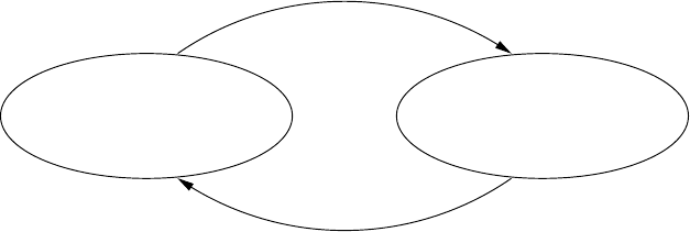
Figure 11.1 illustrates the connection between the forward and the inverse prob-
lem. One also speaks of setting up the forward model y = F(x) and the correspond-
ing inverse model x = F
−1
(y), where y designates the measurement vector and x
is the state vector of the atmosphere to be retrieved.
11.1 Introduction 401
y = F(x)
x = F
−1
(y)
(Estimated) state vector
Vector of measurements
x =(x
1
,...,x
n
) y =(y
1
,...,y
m
)
Fig. 11.1 Forward and inverse problem in remote sensing applications. Note that
the solution to the inverse problem in general provides only an estimate for the
true state of the atmosphere.
For the forward problem the function F can be seen as the RTE. It should be kept
in mind, however, that this is only true for an ideal instrument. In practice, F has to
consider the instrumental properties, such as slit function, response function, field
of view and noise. This means that the forward model has to simulate the instrument
signal by performing a convolution of the radiance spectrum as seen by an ideal
instrument with the various instrument characterizing functions.
While y = (y
1
, y
2
,...,y
m
) is the radiance at the instrument’s location for a set
of m different wavelengths, i.e. a radiance spectrum, the vector x = (x
1
, x
2
,...,x
n
)
could be temperature values T (z
1
), T (z
2
),...,T (z
n
)atn altitudes z
1
, z
2
,...,z
n
.
The determination of a medium’s state based on measured spectra is not limited
to atmospheric applications. Similar problems arise in other disciplines, e.g. the
determination of the composition of the Earth’s interior by exploiting seismic waves,
the derivation of the properties of single stars and galaxies on the basis of radio
waves, infrared or gamma ray observations, or in medicine using nuclear spin
computer tomography, techniques of nuclear medicine or ultrasound. In all these
applications the derivation of the target’s properties and/or composition is called
an inverse problem.
In general it is not possible to exactly reconstruct the state of the target under
investigation. One reason for this is the fact that any measurement contains to some
degree noise signals. Thus the relation y = F(x) is only approximately fulfilled.
Likewise the measurement apparatus may possess certain systematic inaccuracies
which lead to a distorted observation, and the forward model F renders only an
approximate solution to the real problem. Finally, one has to keep in mind that
with a discrete set of observations, that is with a limited number of observations,
402 Remote sensing applications of radiative transfer
one cannot reconstruct field properties of the medium which depend on certain
geophysical parameters in a continuous manner.
In principle, the number n of unknown parameters must be smaller than the num-
ber m of independent measurements, n ≤ m. In the ideal case that each individual
measurement provides an independent piece of information, we would be able to
find a unique solution for the n required parameters. In practice, however, it is not
an easy task to determine the information content of a set of measurements. To give
an example, the observation of the nadir radiance from space in the wavelength
region 290 to 330 nm allows one not only to determine the total column amount
of ozone below the sub-satellite point, it is also possible to ‘sound’ the atmosphere
as a function of increasing distance from the platform if the wavelength is scanned
from smaller to larger wavelengths. This is due to the fact that ozone molecules
absorb solar radiation very strongly at short wavelengths, i.e. photons entering the
atmosphere are not able to pass the ozone layer, with maximum concentration near
20 to 25 km altitude at the short-wave end of this particular wavelength region.
On the other hand, for gradually longer wavelengths the chances will increase that
the photons will reach a greater depth (lower altitude) before absorption occurs.
This particular example illustrates the basic principle of passive (or active) remote
sensing: the spectral absorption or emission characteristics in combination with
the monotonously increasing path length provide a direct link between altitude,
absorber amount and magnitude of the observed radiance.
In the following section we will discuss different topics which are necessary to
understand the principles of remote sensing from satellites. Section 11.2 provides
some insight into solar–terrestrial relations. The physical principles of remote sens-
ing based on the extinction of solar radiation and in the long-wave spectral region
will be described in Section 11.3. In Section 11.4 the inversion of the atmospheric
temperature profile will be analyzed by means of various classical methods. The
final Section 11.5 will make use of the radiative perturbation technique introduced
in Chapter 6 to provide an efficient and accurate algorithm for determining the
so-called weighting function which is of key importance to any physically mathe-
matically based inversion technique.
11.2 Remote sensing based on short- and long-wave radiation
At a wavelength of about 4
µm the spectrum can be separated into the short-wave
region (λ<3.5
µm), where the Sun is the radiation source, and the long-wave
region (λ>3.5
µm), where the thermal emission of the Earth itself and the Earth’s
atmosphere are the sources of radiation. A particularly important wavelength region
is the UV/VIS (UV: ultraviolet, VIS: visible) spectral region in which scattering
of solar radiation by air molecules, aerosol and cloud particles plays an important

11.2 Remote sensing based on short- and long-wave radiation 403
role. An additional feature of the solar radiation can be exploited, namely that both
the diffuse as well as the direct solar radiation can be separately used for remote
sensing.
The different radiation sources lead to different remote sensing algorithms, each
taking advantage of a particular feature of the radiative transfer process. One class
of methods is based on the extinction process, while a second class has its focus on
the scattering process for short-wave radiation. In the long-wave spectral region the
thermal emission as function of the temperature field is in the center of the inves-
tigation. The different methods can also be based on observations from the ground
(ground based), from instruments flown on aircrafts (airborne) or from instruments
aboard rockets or satellites (spaceborne). Regarding satellites, an important obser-
vation geometry is the nadir-looking mode, i.e. the instrument looks at the surface
of the Earth in the nadir direction. Limb sounding means that the viewing path
as seen from the instrument represents a path which is tangential to the Earth
and which, in certain situations, avoids the influence by the Earth’s surface. For
nadir-looking instruments, or instruments covering a wide range of viewing angles,
the contributions of the Earth’s surface play a major role as a function of wave-
length. These contributions are further modified by the radiative properties of the
intervening atmospheric layers. Thus a more or less uniformly distributed (with
respect to wavelength) surface contribution will be modified in a manner that it
carries the spectrally highly variable absorption and emission features of individual
atmospheric trace gases.
11.2.1 Methods based on the extinction of solar radiation
If remote sensing is based on the measurement of short-wave radiation, the follow-
ing assumptions can be made.
(i) The thermal emission source is neglected in the RTE, i.e. J
e
ν
= 0.
(ii) The instrument detects the direct solar radiation only in a very narrow angular solid
angle interval centered around the solar disk. This narrow field of view has the advantage
that contributions due to single or multiple scattering processes of solar photons can
safely be neglected. Thus we can also omit the single and multiple scattering terms in
the RTE.
Introducing these simplifications in the RTE in the form (2.36) we obtain
d
dτ
I
ν
(τ,µ,ϕ) = I
ν
(τ,µ,ϕ) (11.1)
where dτ =−k
ext,ν
ds and s denotes the geometrical distance between P and the
top of the atmosphere in viewing direction of the instrument. Equation (11.1) may
404 Remote sensing applications of radiative transfer
τ
p
τ
m
τ
v
ϑ
0
P
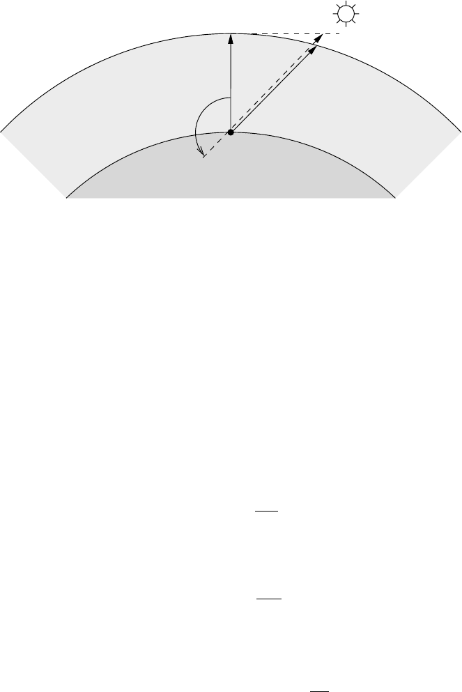
Fig. 11.2 Definition of the optical air mass m for a spherical atmosphere. τ
v
:
vertical optical depth, τ
p
=|µ
0
|
−1
τ and τ
m
= mτ .
be easily integrated yielding
I
ν
(τ,µ,ϕ) = δ(µ − µ
0
)δ(ϕ − ϕ
0
)S
0,ν
exp(−τ
obs
) (11.2)
Here, τ
obs
denotes the optical depth along a straight path between the observation
point P of the instrument and the top of the atmosphere in the direction of the Sun.
Hence, the radiative flux density registered by the instrument is
E
ν
= S
0,ν
exp(−τ
obs
) (11.3)
Since the spectral extraterrestrial solar flux density S
0,ν
is assumed to be known,
the instrument’s signal E
ν
can be used to derive the extinction optical depth of the
entire atmosphere above the observation point
τ
obs
=−ln
E
ν
S
0,ν
(11.4)
Usually one considers the vertical optical depth τ as defined in (2.51). For a
plane–parallel atmosphere we may write
τ
obs
= τ
p
=
τ
|µ
0
|
(11.5)
1
However, since the atmosphere is spherical in nature, τ
obs
is smaller than τ
p
and
is given by
τ
obs
= τ
m
= mτ =
∞
z
k
ext,ν
(z
)
ds
dz
dz
(11.6)
Figure 11.2 depicts the situation.
1
Recall that, according to Figure 2.3, µ
0
≤ 0.