Zdunkowski W., Trautmann T., Bott A. Radiation in the atmosphere: A course in Theoretical Meteorology
Подождите немного. Документ загружается.


7.3 The fitting of transmission functions 245
Having found the k-distribution, we may further define the related cumulative
probability density function g(k) via
g(k) =
k
0
f (k
)dk
(7.177)
In particular we have
g(0) = 0, g(k →∞) = 1, dg(k) = f (k)dk (7.178)
By definition g(k) is a monotone increasing function. Moreover, while for many
gases the spectral absorption coefficient is a highly variable function in ν-space,
its probability density f (k) exhibits much less variation. The reader will not be
surprised when going from f (k)tog(k) that the variability decreases even more
thus leading to a rather smooth cumulative probability density g(k). Having found
g(k), the mean transmission can be obtained from the basic equation (7.163) so that
T
ν
(u) =
ν
exp
(
−k
ν
u
)
dν
ν
=
1
0
exp
[
−k(g)u
]
dg (7.179)
It should be noted that k = k(g) is the inverse function of g = g(k).
Due to the fact that the cumulative probability density function is rather smooth,
the integration over g in (7.179) can be computed very accurately. Often one
employs Gaussian quadrature which means that certain g
j
and w
j
are used for
the abscissa and weights of the quadrature rule. This yields
T
ν
(u) =
1
0
exp
[
−k(g)u
]
dg ≈
J
j=1
w
j
exp[−k(g
j
)u] (7.180)
where J is the total number of quadrature abscissa. Depending on the required accu-
racy of the transmission values one may use, for example, four to fifteen quadrature
nodes.
For demonstration purposes we will now discuss a realistic situation by consid-
ering a spectral interval within the vibration–rotation water vapor band. First we
calculate the absorption spectrum, then we find the frequency distribution f (k) and
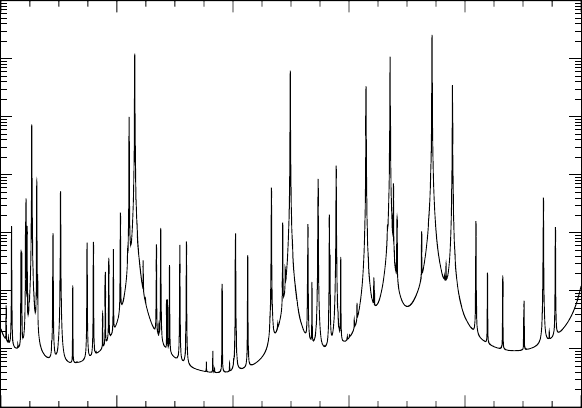
finally the cumulative distribution g(k). Figure 7.10 depicts the spectral absorption
coefficient as calculated by means of line-by-line computations using the spec-
troscopic data for water vapor from the HITRAN database (Rothman et al. 1987,
1992). These computations employ the Voigt profile for the shape of the spectral
lines. In the HITRAN database one can find, among other information, the spectral
position of each spectral line, the line intensity and the half-width for standard
temperature and pressure. Furthermore, one has to describe a cutoff limit beyond
which the contributions of neighboring spectral lines can be neglected. Putting the
information together line-by-line, one arrives at the graph of Figure 7.10.
246 Transmission in spectral lines and bands of lines
1510 1512 1514 1516 1518 1520
10
−4
10
−2
10
0
10
2
k (atm-cm)
−1
(
cm
−1
)
~
ν
Fig. 7.10 Line-by-line calculations of the absorption coefficient for the spectral
range extending from 1510–1520 cm
−1
, p = 10 hPa, T = 240 K. This interval is
located within the vibration–rotation water vapor band.
The units (atm-cm)
−1
of the ordinate are obtained by multiplying the absorp-
tion cross-section for given coordinates ( p, T )byLoschmidt’s number N
L
=
2.6867 × 10
19
cm
−3
. This is the number of molecules per cm
3
of the absorb-
ing gas under standard temperature and pressure conditions. The spectral lines
have been computed on a wave number grid with an extremely fine resolution of
10
−4
cm
−1
. The influence of neighboring lines from outside the selected interval
(1510–1520) cm
−1
has been accounted for by setting the cutoff wave number to
25 cm
−1.
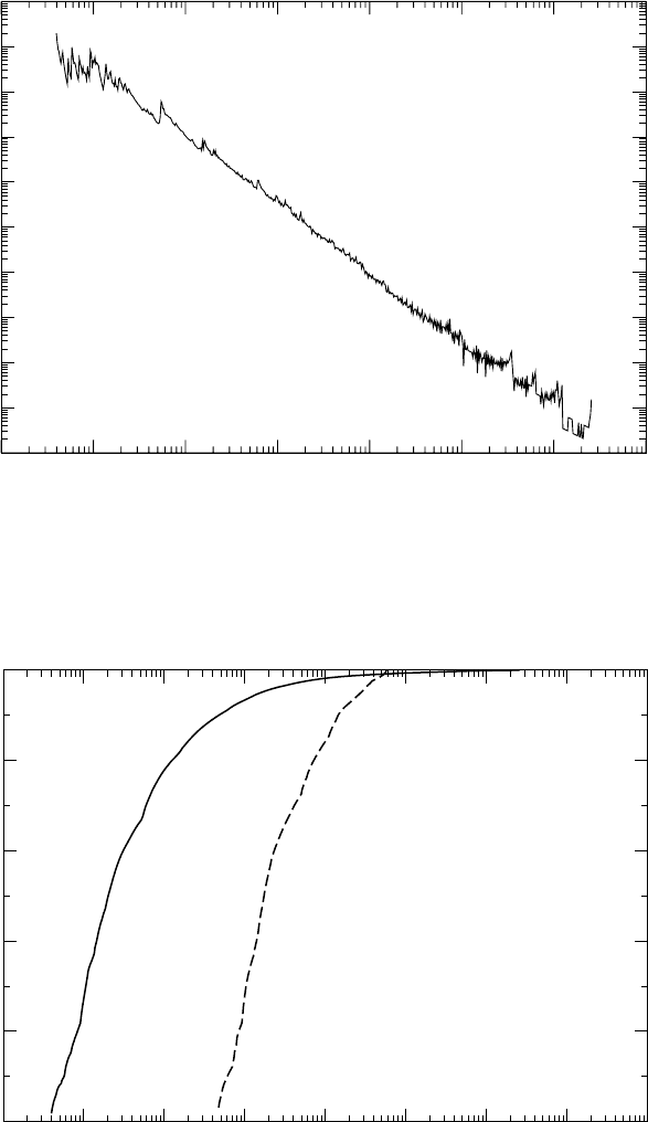
The frequency distribution f (k) corresponding to Figure 7.10 was computed by
binning the k-values into a discrete k-grid employing a total of 100 logarithmically
equidistant k-values per decade of k, see Figure 7.11. A sufficiently fine resolution
(10
−4
cm
−1
in our case) is mandatory in order to obtain a satisfactory f (k) dis-
tribution. A coarser k-binning grid yields the physically unrealistic occurrence of
gaps in the discrete frequency distribution.
Finally, the results of Figure 7.11 were used to compute the cumulative distribu-
tion g(k), as stated in (7.178), see Figure 7.12. While the distribution f (k) exhibits
some structure, the cumulative distribution g(k) is very smooth. The solid line refers
to p = 10 hPa and T = 240 K. For comparison purposes an additional calculation
10
−4
10
−3
10
−2
10
−1
10
0
10
1
10
2
10
3
k (atm-cm)
−1
10
−6
10
−4
10
−2
10
0
10
2
10
4
f(k)
Fig. 7.11 Frequency distribution f (k) of the absorption spectrum shown in
Figure 7.10.
0.0
0.2
0.4
0.6
0.8
1.0
g(k)
k (atm-cm)
−1
10
−4
10
−2
10
0
10
2
10
4
Fig. 7.12 Cumulative frequency distribution g(k) for two combinations of (p, T ).
Solid line: p = 10 hPa, T = 240 K, dashed line: p = 1000 hPa, T = 296 K.

248 Transmission in spectral lines and bands of lines
was carried out for p = 1000 hPa, T = 296 K which is displayed by the dashed
curve.
7.3.3 The correlated k-distribution method
So far our derivations for the k-distribution method are valid only for homogeneous
atmospheres. The extension to a realistic, inhomogeneous atmosphere requires
some careful considerations. Here we follow the discussion of Fu and Liou (1992)
and introduce the concept of correlated k-distributions. First, we have to recall the
dependence of k
ν
on temperature and pressure
k
ν
=
i
S
i
(T ) f
i
(ν, p, T ) (7.181)
where the summation indicates that several spectral lines may contribute to the
value of the absorption coefficient at a particular wave number ν. The S
i
and f
i
are
the line intensities and the line-shape factors of the lines, respectively.
If we want to apply the k-distribution method to an inhomogeneous atmosphere,
we will consider an atmospheric layer defined by the heights z
1
and z
2
> z
1
. The
mean transmission for this layer can be obtained from
T
ν
(u) =
1
ν
ν
exp
−
z
2
z
1
k
ν
(p, T )ρ
abs
dz
dν (7.182)
where ρ
abs
is the density of the absorbing gas.
Now we will discuss the mathematical and physical requirements under which
(7.182) can be replaced by a form similar to (7.179), i.e.
T
ν
(u) =
1
0
exp
−
z
2
z
1
k(g, p, T )ρ
abs
dz
dg (7.183)
If the mean transmission is computed according to (7.183), then the k-distribution
approach is referred to as the correlated k-distribution (CKD) method.
Since pressure and temperature vary over the layer (z
1
, z
2
), we should expect
that for different levels in the atmosphere there are different g = g(k) relationships
for the same wave number ν. In fact, this general behavior is not what the CKD
method assumes. Here we make the assumption that despite varying pressure and
temperature there is only one g value for a particular ν at all levels of the inhomoge-
neous atmosphere. For this to be fulfilled, we first must assume that the absorption
coefficients at two wave numbers ν
1
and ν
2
are the same for any p and T , if they
are the same at the reference state (p
r
, T
r
)
k(ν
1
, p
r
, T
r
) = k(ν
2
, p
r
, T
r
) =⇒ k(ν
1
, p, T ) = k(ν
2
, p, T )
(7.184)
We will call this the first requirement for the CKD method.

7.3 The fitting of transmission functions 249
If (7.184) is assumed to be valid for an arbitrary wave number ν we may conclude
that the spectral absorption coefficient for arbitrary ν, p and T may be cast into the
functional form
k(ν, p, T ) = χ
[
k
r
(ν), p, T
]
with k
r
(ν) = k(ν, p
r
, T
r
) (7.185)
where the function χ consists of a ν-dependent part which can be separated from
the ( p, T )-dependence. Since in (7.185) there appears only a single reference func-
tion k
r
(ν), we may compute the corresponding probability density function f
r
(k).
Introducing (7.185) into (7.182) and transforming to the k-space, we obtain
T
ν
(u) =
∞
0
exp
−
z
2
z
1
χ(k
r
, p, T )ρ
abs
dz
f (k
r
)dk
r
(7.186)
Assuming that for the reference condition g
r
(k
r
) is a monotonic function of k
r
,we
may also compute the relationship k
r
= k
r
(g
r
). Thus, in g
r
-space the function χ
may be identified with another function β which depends on g
r
χ
[
k
r
(g
r
), p, T
]
= β
(
g
r
, p, T
)
(7.187)
Using the last definition and (7.178), the mean transmission for the layer (z
1
, z
2
)
can be computed from
T
ν
(u) =
1
0
exp
−
z
2
z
1
β(g
r
, p, T )ρ
abs
dz
dg
r
(7.188)
As the second requirement for the CKD approach we postulate that
k(ν
i
, p
r
, T
r
) > k(ν
j
, p
r
, T
r
) =⇒ k(ν
i
, p, T ) > k(ν
j
, p, T )
(7.189)
This assumption has an important consequence. The ordering of the spectral absorp-
tion coefficients, as required for the computation of the cumulative probability dis-
tribution, is independent of the actual values of pressure and temperature. In other
words, there exists only one g for a given wave number ν at different atmospheric
levels, that is
g
r
[
k
r
(ν)
]
= g
[
k(ν, p, T ), p, T
]
(7.190)
This last relation can be used to find the mean transmission for layer (z
1
, z
2
)by
means of a single g function
T
ν
(u) =
1
0
exp
−
z
2
z
1
β(g, p, T )ρ
abs
dz
dg (7.191)

250 Transmission in spectral lines and bands of lines
By using equations (7.185), (7.187) and (7.190) we may conclude that the two
requirements of the CKD method lead to the relationship
k = β
[
g(k)
]
(7.192)
If k is a monotone function in g-space, then β(g) = k(g) as follows from differen-
tiating (7.192) with respect to k. This last identity makes (7.191) to be equivalent
to (7.183).
The first requirement of the CKD method provides the basis for using the k-
distribution method at the reference state ( p
r
, T
r
). The second requirement relates
the cumulative probability function of the reference state to any other level, i.e. for
other values of p, T .
7.3.4 The k-distribution method for special situations
Two overlapping gases
For certain gases it is necessary to treat overlap effects in radiative transfer cal-
culations. Due to the fact that computational speed is a very important issue in
radiative transfer modeling, in particular for vertically inhomogeneous scattering
and absorbing atmospheres, a fast method must be provided allowing the treatment
of overlapping effects in an efficient manner.
The mean transmission of two different gases 1 and 2 in a wave number interval
of width ν is defined as
T
ν
(1, 2) =
1
ν
ν
T
ν
(1)T
ν
(2)dν (7.193)
To simplify this expression we assume that the spectral transmissions of the gases
are uncorrelated. This implies that the mean of the product of the individual trans-
missions equals the product of the corresponding mean transmissions, i.e.
T
ν
(1, 2) = T
ν
(1)T
ν
(2) (7.194)
Expressing the individual transmissions for the layer (z
1
, z
2
)ing-space as
T
ν
(i) =
1
0
exp
−
z
2
z
1
k
i
ρ
abs,i
dz
dg
i
, i = 1, 2 (7.195)
the mean transmission of the two overlapping gases can be formulated as
T
ν
(1, 2) =
1
0
1
0
exp
−
z
2
z
1
[k
1
ρ
abs,1
+ k
2
ρ
abs,2
]dz
dg
1
dg
2
≈
M
m=1
N
n=1
exp(−τ
mn
)g
1m
g
2n
(7.196)
7.3 The fitting of transmission functions 251
where ρ
abs,1
, ρ
abs,2
and k
1
, k
2
are the density and the absorption coefficient of gas
1 and gas 2, respectively. The optical depth of the two gases in the layer is defined
by
τ
mn
=
z
2
z
1
[k
1
ρ
abs,1
+ k
2
ρ
abs,2
]dz (7.197)
In summary we conclude, that for obtaining the absorption effect of two gases
which overlap in a particular wave number interval, we must carry out M × N
quasi-spectral radiative transfer calculations for each vertical atmospheric column.
To give an example of the amount of computations involved, let us consider the
overlap of CO
2
and H
2
O in the spectral region 540–800 cm
−1
. Fu and Liou (1992)
recommend in their CKD method a subdivision of this region into the two subregions
540–670 cm
−1
and 670–800 cm
−1
. In the first subregion they employ for H
2
O and
CO
2
an expansion with 5 and 10 terms, respectively. In the second subinterval the
corresponding numbers are 4 (H
2
O) and 8 (CO
2
). Hence a total of 5 ×10 + 4 × 8 =
82 quasi-monochromatic radiative transfer computations has to be performed. This
illustrates the increased computational effort involved when treating gas overlap
effects in atmospheric radiative transfer. Additional simplifications can be used to
reduce computational efforts. For more details the reader is invited to consult the
original papers.
Gray absorption coefficient
We consider the wave number range ν, in which the absorption coefficient takes
on the constant value k
ν
=
¯
k. According to (7.163) the k-distribution is then given
by
f (k) = δ(k −
¯
k) (7.198)
where δ(k −
¯
k) is the Dirac δ-function.
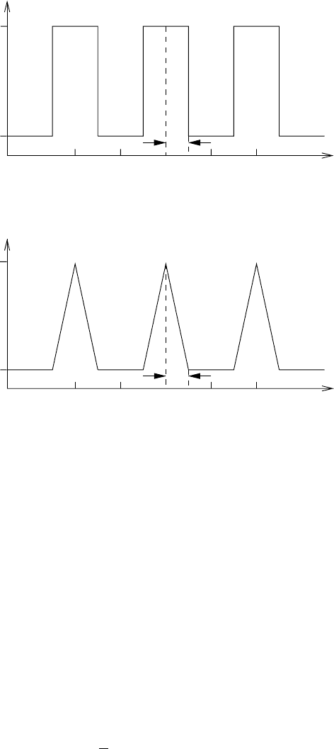
Regular band of nonoverlapping rectangular lines
The next example is a regular band of an infinite number of nonoverlapping rectan-
gular lines. Let b represent the half-width of the rectangular line and define α = b/δ.
The absorption coefficient is then given by
k
ν
=
k
1
for α ≤ ν/δ ≤ 1/2
k
2
for 0 ≤ ν/δ ≤ α
(7.199)
For this spectral arrangement we read from Figure 7.13
f (k) = (1 − 2α)δ(k − k
1
) + 2αδ(k − k
2
) (7.200)
252 Transmission in spectral lines and bands of lines
−1 −0.5 0 0.5 1
k
1
k
2
k
ν
x
α
Fig. 7.13 A regular band of nonoverlapping rectangular lines with x = ν/δ.
−0.5 0 0.5 1 −1
k
1
k
2
x
k
ν
α
Fig. 7.14 A regular band of nonoverlapping triangular lines with x = ν/δ.
For the mean absorption coefficient we obtain by inspection of Figure 7.13 the
relation
¯
k = k
1
+ 2α(k
2
− k
1
) (7.201)
Alternatively, we can calculate the mean absorption coefficient from the k-
distribution
¯
k =
∞
0
kf(k)dk =
∞
0
k(1 − 2α)δ(k − k
1
)dk +
∞
0
2αkδ(k − k
2
)dk
= (1 − 2α)k
1
+ 2αk
2
= k
1
+ 2α(k
2
− k
1
)
(7.202)
Regular band of triangular lines
In this case the absorption coefficient is given by, see Figure 7.14
k
ν
=
/
k
2
−
ν
α
(k
2
− k
1
) for 0 ≤ ν/δ ≤ α
k
1
for α ≤ ν/δ ≤ 1/2
(7.203)
7.3 The fitting of transmission functions 253
−
0.5 0 0.5
1 −1
k
1
k
2
k
ν
x
α
L
Fig. 7.15 A regular band of nonoverlapping Lorentz lines with x = ν/δ.
A few simple algebraic steps lead to
f (k) = (1 − 2α)δ(k − k
1
) +
2α
k
2
− k
1
for k
1
≤ k ≤ k
2
0 for k < k
1
or k > k
2
(7.204)
For the average absorption coefficient we obtain
¯
k =
∞
0
kf(k)dk = k
1
(1 − 2α) +
2α
k
2
− k
1
k
2
2
k
2
k
1
= k
1
+ α(k
2
− k
1
)
(7.205)
This result also follows directly from inspection of Figure 7.14.
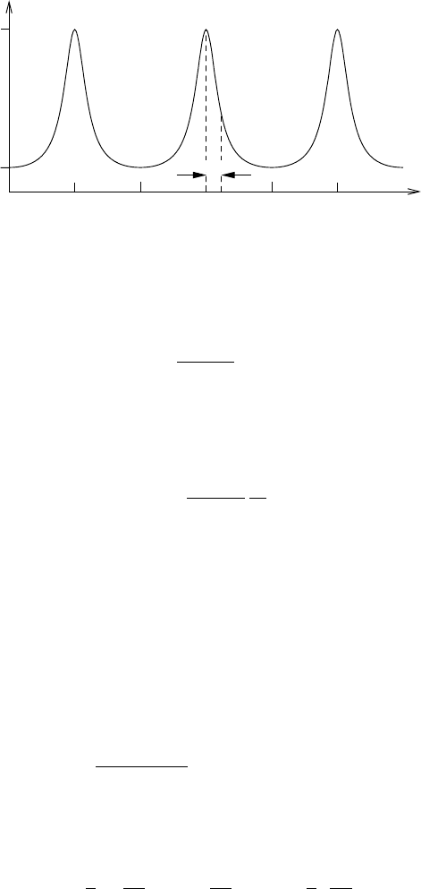
Regular band of nonoverlapping Lorentz lines
As a final example we discuss a situation which is similar to the regular Elsasser
model. However, there is one exception, namely that the individual identical Lorentz
lines are cut off at the distance δ/2 from each center line, see Figure 7.15.
In this case we have
k
ν
=
Sα
L
π
ν
2
+ α
2
L
for 0 ≤ ν ≤ δ/2 (7.206)
With this information we employ (7.168) to find f (k) by differentiation
f (k) =
1
δ
dν
dk
ν
1
+
dν
dk
ν
2
=
2
δ
dν
dk
ν
2
(7.207)
where ν
1
= (−δ/2, 0) and ν
2
= (0,δ/2). The last step follows from
symmetry. The expression for the spectral absorption coefficient can be directly
254 Transmission in spectral lines and bands of lines
solved for ν yielding
ν =
%
Sα
L
πk
− α
2
L
(7.208)
Computing the first derivative of ν with respect to k, we obtain
dν
dk
=−
1
2
$
Sα
L
/(πk) − α
2
L
Sα
L
πk
2
(7.209)
Substituting the maximum value of the absorption coefficient k
2
= S/πα
L
gives
dν
dk
=
1
2
k
2
α
L
k
3/2
√
k
2
− k
(7.210)
Thus we find the k-distribution of the cut-off Lorentz band in the form
f (k) =
k
2
α
L
δk
3/2
√
k
2
− k
(7.211)
From
¯
k =
kf(k)dk we obtain after some tedious but straightforward steps
¯
k =
2k
2
α
L
δ
tan
−1
δ
2α
L
(7.212)
Details in the derivation will be left up to the exercises.
Single scattering properties for inhomogeneous atmospheres
While gaseous atmospheric absorption is described by the spectral absorption coef-
ficient, extinction by air molecules, aerosol particles and hydrometeors requires
additional information on the extinction coefficient, the single scattering albedo
and the scattering phase function. Below we will describe how these radiative
properties are combined to yield the scattering and absorption properties of an indi-
vidual homogeneous atmospheric layer embedded in an otherwise inhomogeneous
atmosphere.
We will assume that the inhomogeneous atmosphere consists of a set of distinct
homogeneous layers. For a certain wave number band ν the total optical depth of
a layer z consists of Rayleigh scattering τ
R
, Mie scattering due to atmospheric
aerosol particles and hydrometeors τ
M
, and the contribution τ
G
due to gas
absorption
τ = τ
R
+ τ
M
+ τ
G
(7.213)
Absorption by a gas with density ρ
abs
may be described by means of the CKD
approach yielding
τ
G
(g) = k(g)ρ
abs
z (7.214)