Zdunkowski W., Trautmann T., Bott A. Radiation in the atmosphere: A course in Theoretical Meteorology

Подождите немного. Документ загружается.

4.3 The discrete ordinate method 95

(1) Each iteration step has a physical signiﬁcance, i.e. each additional iteration means that

one additional scattering process is simulated.

(2) The inhomogeneity of the optical parameters can be easily handled, that is – in contrast

to the MOM – an a priori subdivision of the atmosphere into different individual

homogeneous sublayers is not necessary.

However, the SOS method has the disadvantage of requiring a large number of

iteration steps thus converging very slowly. This is particularly true if the medium

is practically conservative (ω

→ 1) or if it has a very large optical thickness. In

these situations, however, techniques for speeding up the convergence process may

partly eliminate the problem.

The SOS method in the form described above follows an unpublished lecture

given by Z. Sekera. A detailed description is given in Korb and Zdunkowski (1970).

A fairly complete list of references for SOS may be found in Lenoble (1985).

4.3 The discrete ordinate method

The discrete ordinate method (DOM) is another very elegant approach for solving

the RTE in a plane–parallel atmosphere. It also belongs to the most accurate tech-

niques and may be used for calculating benchmark solutions to certain problems.

The formulation of the DOM dates back to Chandrasekhar (1960). Starting point

for the DOM is the discretization of the m-th Fourier mode of the radiance ﬁeld,

see (2.69).

In the following we discuss the DOM for the azimuthally averaged radiation

ﬁeld, i.e. for m = 0. Only the case m = 0 is needed to calculate important quantities

such as radiative ﬂux densities, actinic ﬂuxes, and heating rates. Actinic ﬂuxes are

important for photochemistry and result from integrating the radiance over the unit

sphere. The case m = 0 is needed to account for the directional dependence of

the radiation ﬁeld as required, for example, in remote sensing. In the sequel, for

m=0

(τ,µ) we will simply write I (τ,µ). From (2.76) it may be seen that for the

case m = 0 the same procedure applies.

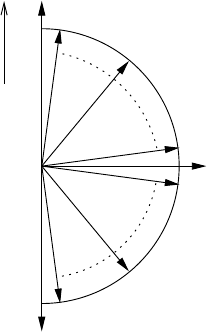
Let us consider a total of 2s directions for discretizing the radiation streams,

that is −1 ≤ µ

≤ 1, i =−s,...,−1, 1,...,s, as illustrated in Figure 4.5. In the

following it will be shown how to solve analytically the resulting coupled system

of linear differential equations for homogeneous sublayers.

Evaluating (2.76) for m = 0 at the discrete direction µ

and approximating the

multiple scattering integral with the help of the Gaussian quadrature (2.88) leads to

dI(τ,µ

)

dτ

= I (τ, µ

) −



j=−s



I (τ,µ

)P(µ

,µ

)

−

4π

exp



−



P(µ

, −µ

) − (1 − ω

)B(τ ) (4.31)

96 Quasi-exact solution methods for the RTE

µ = −1

µ =0

µ =1

−

−s

Fig. 4.5 Discretization of I (τ,µ) in a total of 2s streams.

where the azimuthally averaged phase function P(µ, µ



) has been used as deﬁned

in (2.80). For practical reasons the inﬁnite series in (2.80) must be truncated after a

sufﬁcient number of terms. The special case that the direction µ

of the direct solar

beam coincides with one of the quadrature directions must be avoided, otherwise

singularities would occur.

From (2.88) it may be easily seen that the Gaussian quadrature of order r is exact

on the interval [−1, 1] for Legendre polynomials P

(µ), m = 0, 1,...,2r − 1,

that is



−1

(µ) dµ =



i=1

(µ

) = 2δ

, m = 0, 1,...,2r − 1 (4.32)

An important consequence of this is that the normalization condition of the phase

function (2.62) is also satisﬁed in its discretized version when developing this

function into a ﬁnite series of Legendre polynomials which is truncated after the

term l = 2r − 1. We will now demonstrate this. Starting with (2.68) we ﬁnd the

following expression

P(cos ) =

2r−1



l=0

(cos )

2r−1



l=0

(µ)P

(µ



) + 2

2r−1



m=1

2r−1



l=m

(µ)P

(µ



) cos m(ϕ − ϕ



)

= P(µ, µ



) + 2

2r−1



m=1

2r−1



l=m

(µ)P

(µ



) cos m(ϕ − ϕ



) (4.33)

4.3 The discrete ordinate method 97

To see that there is no need to renormalize the phase function in DOM, consider

the quadrature form of the normalization condition as applied to P(µ, µ



)



−1

P(µ, µ



) dµ





i=1

P(µ, µ

)



i=1

2r−1



m=0

(µ)P

(µ

)

2r−1



m=0

(µ)



i=1

(µ

) (4.34)

2r−1



m=0

(µ)



−1

(µ) dµ

2r−1



m=0

(µ)δ

= 1

As demonstrated by Wiscombe (1977), the above property also holds for the

so-called δ-scaled phase function P

∗

(µ, µ



) as deﬁned by

∗

(µ, µ



) = 2 f δ(µ − µ



) + (1 − f )

2r−1



m=0

∗

(µ)P

(µ



)

(4.35)

if it is truncated after the term l = 2r − 1. The quantity f is the fraction of radiation

scattered into the forward peak of the phase function. We refrain from proving this

equation since the proof is carried out analogously to the development leading to

(4.34). Note also that p

= p

∗

. The δ-scaled phase function will be discussed in

more detail in a later chapter.

If the expansion of the phase function is continued beyond 2r − 1 then the phase

function is no longer correctly normalized so that artiﬁcial absorption may occur as

pointed out by Wiscombe (1977). It is important to realize that the normalization of

the phase function is a basic requirement for the numerical algorithm to be energy

conserving.

An additional comment is due regarding an improved discretization of the

term I (τ, µ) =



−1

I (τ,µ



)P(µ, µ



) dµ



. The ordinary Gaussian quadrature, used

before, reads



−1

I (τ,µ



)P(µ, µ



) dµ



≈



i=−n



I (τ,µ

)P(µ, µ

) (4.36)

For increasing quadrature order n the nodes µ

still cluster near µ = 1 and µ =−1,

but only a few nodes are located near the horizon µ = 0. Therefore, for strongly

anisotropic phase functions the accuracy of the radiance ﬁeld does not improve

98 Quasi-exact solution methods for the RTE

signiﬁcantly by simply increasing the number of nodes. In order to improve this

situation one can use a simple trick by splitting the integration over [−1, 1] into

the subintervals [−1, 0] and [0, 1]. By using the transformations ˜µ = 2µ + 1 for

the interval [−1, 0] and ˜µ = 2µ − 1 for the interval [0, 1] and applying a s-point

Gaussian quadrature, we can write for integrals of the type



−1

f (µ) dµ =



−1



˜µ − 1



d ˜µ +



−1



˜µ + 1



d ˜µ

≈



i=1





˜µ

− 1



+ f



˜µ

+ 1



(4.37)

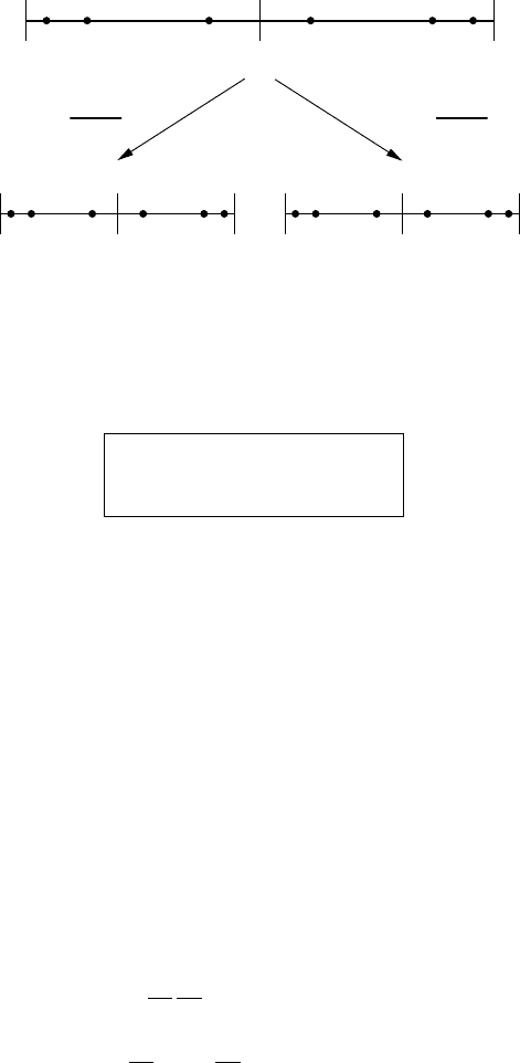
Figure 4.6 illustrates how the ordinary s-point Gaussian quadrature for the vari-

able ˜µ is mapped onto the intervals [−1, 0] and [0, 1] for the variable µ. The latter

nodes are now symmetric with respect to the locations µ =−0.5 and µ = 0.5 and

cluster near the end points of each interval. It can also be seen that the nodes µ

are

antisymmetric with respect to µ = 0.

The zeros and weights of the Legendre polynomials occurring in (4.37) have the

following properties

˜µ

=−˜µ

s+1−i

, w

= w

s+1−i

, i = 1,...,s (4.38)

Utilizing these expressions together with the substitution µ



= (˜µ

+ 1)/2, the

right-hand side of (4.37) may be written as



i=1





˜µ

− 1



+ f



˜µ

+ 1





i=1





−

˜µ

s+1−i

+ 1



+ f



˜µ

+ 1





i=1

s+1−i



−µ



s+1−i





i=1









i=1





−µ





+ f







(4.39)

Introducing the nodes µ



and weights w



according to



, w



−i

= w



˜µ

+ 1

, µ



−i

=−µ



i = 1,...,s

(4.40)

4.3 The discrete ordinate method 99

µ =

µ − 1

µ =

µ +1

µ′

−10 1

−1

−0.5 0.5010

Fig. 4.6 The double-Gaussian quadrature rule. The dots mark the locations of the

quadrature nodes for i = 1,...,s.

results in the so-called double-Gaussian quadrature of order 2s



−1

f (µ) dµ ≈



i=−s



f (µ



)

(4.41)

Recall that the notation





means that in the summation the term i = 0 is omitted.

Hence for the 2s-point double-Gaussian quadrature formula only the nodes and

zeros (w

,µ

) of the original s-point Gaussian quadrature formula are needed.

The advantage of the double-Gaussian quadrature formulas is that the nodes are

not only clustered in both the upward and downward directions but also near the

horizon.

Let us now ﬁnd the solution to the RTE for the special case that no thermal

emission exists, B(τ ) = 0. Inclusion of this term, however, poses no particular

difﬁculty. The treatment of thermal emission will be taken care of in a later chapter.

For a layer with constant optical properties the inhomogeneous system of linear

differential equations (4.31) can be solved exactly. The solution is composed of

the general solution of the homogeneous system plus a particular solution of the

inhomogeneous part. First let us deﬁne the set of coefﬁcients

i, j











−

P(µ

,µ

) i = j



1 −

P(µ

,µ

)



i = j

(4.42)

These coefﬁcients satisfy the asymmetry relations

i, j

=−b

−i,−j

, b

i,−j

=−b

−i, j

(4.43)

100 Quasi-exact solution methods for the RTE

The homogeneous part of (4.31) can then be written as

dI(τ,µ

)

dτ



j=−s



i, j

I (τ,µ

) (4.44)

If we distinguish between upwelling and downwelling radiation, then from (4.44)

we obtain

dI(τ,µ

)

dτ



j=1

i, j

I (τ,µ

) +



j=1

i,−j

I (τ,−µ

)

dI(τ,−µ

)

dτ



j=1

−i, j

I (τ,µ

) +



j=1

−i,−j

I (τ,−µ

)

(4.45)

which can be written in vector–matrix form as

dτ



−





−

−B

−

−B



−



(4.46)

Here the vectors I

and the matrices B

are deﬁned as







I (τ,±µ

)

I (τ,±µ

)







= (b

i, j

)

−

= (b

i,−j

)

i = 1,...,s

j = 1,...,s

(4.47)

With the exponential trial solution

= F

exp(−kτ ) (4.48)

involving the vectors F

= (F

±,i

), i = 1,...,s which are independent of τ , the

homogeneous system (4.46) may be transformed into an eigenvalue problem of

order 2s



−

−B

−

−B



−



=−k



−



(4.49)

Without going into details we need to mention that all eigenvalues occur in pairs

±k (see Chandrasekhar, 1960) and that they are all real (Kuˇsˇcer and Vidav, 1969).

Due to the particular form of the nonsymmetrical matrices B

−

and B

the above

eigenvalue problem of order 2s can be reduced to a corresponding problem of order

s as will be shown next. Adding and subtracting the ﬁrst and second equation in

(4.49) leads to

(a)

(

− B

−

)(

− F

−

)

=−k

(

+ F

−

)

(b)

(

+ B

−

)(

+ F

−

)

=−k

(

− F

−

)

(4.50)

4.3 The discrete ordinate method 101

If we now multiply (4.50b) by (B

− B

−

) and insert on the right-hand side of the

resulting expression (4.50a), we obtain

(

− B

−

)(

+ B

−

)(

+ F

−

)

= k

(

+ F

−

)

(4.51)

Thus we obtain an eigenvalue problem of order s involving the matrix (B

−

)(B

+ B

−

) with eigenvalues k

and eigenvectors F

+ F

−

. We may then use

(4.50b) to determine F

− F

−

. The eigenvectors F

, F

−

of the original equation

(4.49) can be found from

= F

+ F

−

, X

−

= F

− F

−

(

+ X

−

)

, F

−

(

− X

−

)

(4.52)

As mentioned above, the 2s eigenvalues of (4.49) are all distinct and occur in pairs

±k

,(j = 1,...,s). These eigenvalues and the corresponding i-th component of

the j-th eigenvector, F

(µ

), for eigenvalue k

can be efﬁciently computed with

numerical standard algorithms (see, e.g. Press et al., 1992).

The general solution I

of the homogeneous system is then given by

(τ,µ

) =



j=−s



(µ

) exp(−k

τ ), i =−s,...,−1, 1,...,s (4.53)

The constants D

, j =−s,...,−1, 1,...,s follow from the boundary conditions

at the upper and the lower boundary of the homogeneous layer.

A particular solution I

of the inhomogeneous system can be obtained from a

trial solution resembling the functional form of the right-hand side of (4.31)

(τ,µ

) = Z (µ

)exp



−



, i =−s,...,−1, 1,...,s (4.54)

where the 2s unknown coefﬁcients Z(µ

), i =−s,...,−1, 1,...,s can be found

by inserting (4.54) into (4.31). In summary, for a homogeneous layer the complete

solution of the azimuthally averaged RTE can now be written down by adding the

homogeneous solution (4.53) and the inhomogeneous solution (4.54) yielding

I (τ,µ

) =



j=−s



(µ

) exp(−k

τ ) + Z (µ

)exp



−



(4.55)

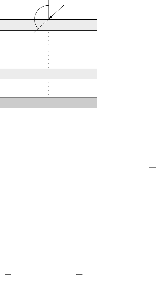
So far we have considered the particular case of a single homogeneous layer. The

inhomogeneous atmosphere will now be subdivided into Q different homogeneous

sublayers, see Figure 4.7. The complete solution for each homogeneous sublayer

102 Quasi-exact solution methods for the RTE

Layer

Optical depth

0,1

0,q

Ground A

∆τ

q−1

Fig. 4.7 Subdivision of the atmosphere in a total number of Q different homo-

geneous sublayers with optical thickness τ

, single scattering albedo ω

0,q

and phase function P

, q = 1,...,Q. The albedo of the diffusely reﬂecting

ground is A

is already known from (4.55). For layer q we now write

(τ,µ

) =



j=−s



q, j

(µ

) exp[−k

q, j

(τ − τ

q−1

)] + Z

(µ

)exp



−



(4.56)

with 1 ≤ q ≤ Q. Note that in the homogeneous part of the solution the integration

constants D

q, j

, the eigenvalues k

q, j

, the components of the eigenvectors F

q, j

, and

the constants Z

of the particular solution refer to layer number q. It is also clear

that the solution (4.56) is only valid for the optical depth τ

q−1

≤ τ ≤ τ

In total 2sQ equations are required to determine the integration constants D

q, j

Two of these equations are given by the speciﬁcation of the boundary conditions at

τ = 0 and τ = τ

. Assuming isotropic reﬂection at the ground with albedo A

obtain

(τ = 0, −µ

) = 0

(τ

,µ

) =



−,z

(τ

) + µ

exp



−





2π



j=1

(τ

, −µ

)µ

+ µ

exp



−



, i = 1,...,s

(4.57)

The upwelling radiance at the ground is assumed to be isotropic and, therefore,

is identical for all directions µ

as expressed by the last equation of (4.57). The

remaining 2(s − 1)Q equations are determined by the requirement that the radiance

4.3 The discrete ordinate method 103

for each µ

must be continuous at each level interface τ

,(q = 1,...,Q − 1), i.e.

(τ

,µ

) = I

q+1

(τ

,µ

), q = 1,...,Q − 1, i =−s,...,−1, 1,...,s

(4.58)

Inserting the complete solution as stated by (4.56) into relations (4.57) and (4.58)

then leads to a linear system for the coefﬁcients D

q,i



j=−s



1, j

(−µ

) =−Z

(−µ

), i = 1,...,s



j=−s



q, j

(µ

) − D

q+1, j

(µ

)] = η

(µ

i = 1,...,s

q = 1,...,Q − 1



j=−s



Q, j

(µ

) =−ε(µ

), i = 1,...,s

(4.59)

where the following abbreviations have been introduced

q, j

(µ

) = F

q, j

(µ

) exp[−k

q, j

(τ

− τ

q−1

)]

(µ

) = [Z

q+1

(µ

) − Z

(µ

)] exp



−



(µ

) =



Q, j

(µ

) − 2A



l=1

Q,l

(−µ

)µ



exp[−k

Q, j

(τ

− τ

Q−1

)]

ε(µ

) =



(µ

) − 2A



j=1

(−µ

)µ

−



exp



−



(4.60)

The linear equation system (4.59) may also be written in matrix form as

KD = X (4.61)

K is a square matrix of dimension (2sQ × 2sQ), and the vectors D and X are 2sQ-

dimensional. From this system of linear equations for 2sQ unknown coefﬁcients

we may obtain the required constants of integration D

q, j

by numerical inversion.

The major advantages and disadvantages of the DOM are listed here.

(1) The solution of the RTE can be derived in a completely explicit form.

(2) The computational effort for each individual layer is independent of its optical depth.

(3) The accuracy of the method compares well with the MOM and, therefore, DOM can

also be used to perform benchmark calculations.

(4) Unless one uses a δ-approximation to the phase function, see (4.35), sharp phase func-

tions may produce unrealistic oscillating radiance patterns.

(5) DOM is computationally too expensive for routine calculations in climate models.

104 Quasi-exact solution methods for the RTE

The DOM in the form described above mainly follows the derivation given in

Stamnes et al. (1988). These authors also supplied the very reliable programme

package DISORT to the scientiﬁc community, a package which is widely used

for various applications. The discretization of the radiance ﬁeld into streams trav-

eling along the directions of the Gaussian quadrature nodes is fully described in

Chandrasekhar (1960). Important developments regarding both the algorithmic for-

mulation of the DOM for an inhomogeneous atmosphere as well as the correct

evaluation of the numerical eigenvalue-eigenvector problem have been contributed

by Liou (1973) and Asano (1975).

4.4 The spherical harmonics method

In this section we will discuss the principles of the spherical harmonics method

(SHM) and illustrate the solution of the radiance ﬁeld for a homogeneous atmo-

spheric layer. The SHM employs the transfer equation (2.76) which is based on the

cosine Fourier expansion of the radiance

I (τ,µ,ϕ) =





m=0

(2 − δ

(τ,µ) cos mϕ (4.62)

There are several equivalent ways of separating the µ and τ dependencies. Here

we choose the following expansion

(τ,µ) =



l=m

2l + 1

(τ )P

(µ) (4.63)

with M = 2p − 1 +m, where p is chosen as the smallest integer number that fulﬁlls

the condition 2p − 1 + m ≥ . Recall also that, according to (2.59a), P

(µ) = 0

for m > l. Inserting (4.63) into (2.76) and employing the integral operation



−1

...P

(µ) dµ (4.64)

leads to a system of  + 1 ordinary inhomogeneous linear differential equations.

Each such system contains 2 p = M + 1 − m differential equations for the deter-

mination of the unknown functions I

(τ ) and has the form

(l + m + 1)

l+1

(τ )

dτ

+ (l − m)

l−1

(τ )

dτ

[

− (2l + 1)

]

(τ )

=−

2π

exp



−



(−µ

) − 2(1 − ω

)B(τ )δ

(4.65)