Zdunkowski W., Trautmann T., Bott A. Radiation in the atmosphere: A course in Theoretical Meteorology
Подождите немного. Документ загружается.


3.4 The inclusion of surface reflection 75
It is possible to extend the analysis to include the effects of polarization. Without
going into details at this point, the scattering and transmission functions S and T
will have to be replaced by scattering and transmission matrices. This makes the
analysis quite complicated. In a later chapter we are going to show how to include
polarization in the radiative transfer equation.
We will conclude this section with a few additional remarks of how to evaluate
the preceding equations by expanding the scattering and transmission functions in
Fourier type series. In Section 2.4 we have shown that if the phase function can be
expressed in the form (2.68), then it is possible to expand the radiance I (τ, µ,ϕ)
by means of (2.69). Similarly, by expanding the phase function in the form (2.68),
the scattering and the transmission functions may be written as
S(τ
1
,µ,ϕ,µ
0
,ϕ
0
) =
N
m=0
S
m
(τ
1
,µ,µ
0
) cos m(ϕ − ϕ
0
)
T (τ
1
,µ,ϕ,µ
0
,ϕ
0
) =
N
m=0
T
m
(τ
1
,µ,µ
0
) cos m(ϕ − ϕ
0
)
(3.38)
By substituting these expansions into (3.36), using the proper orthogonality condi-
tions, we can eliminate the azimuthal dependence. We will not carry out the analysis
but refer the interested reader to Chandrasekhar (1960).
3.4 The inclusion of surface reflection
The boundary conditions (3.30) of the standard problem did not include the effects
of surface reflection which may be of great importance in a number of realistic
situations. Whenever the surface reflection is included in the transfer analysis, we
speak of the planetary problem. To simplify the analysis of the planetary problem,
we will assume that the light is reflected according to Lambert’s law, that is the
reflected light is uniform and independent of the angular distribution of the incoming
light. In this case we also speak of a Lambertian surface. For convenience, as before,
we set the azimuthal angle of the Sun ϕ
0
= 0. Furthermore, we ignore the effects
of polarization.
The two azimuthal independent terms S
0
(τ
1
,µ,µ
0
) and T
0
(τ
1
,µ,µ
0
)inthe
expansions (3.38) are given by
S
0
(τ
1
,µ,µ
0
) =
1
2π
2π
0
S(τ
1
,µ,ϕ,µ
0
, 0)dϕ
T
0
(τ
1
,µ,µ
0
) =
1
2π
2π
0
T (τ
1
,µ,ϕ,µ
0
, 0)dϕ
(3.39)

76 Principles of invariance
To obtain a simple mathematical structure of the equations to be derived, we intro-
duce the abbreviations
(a) s(τ
1
,µ) =
1
2
1
0
S
0
(τ
1
,µ,µ
)dµ
(b) t(τ
1
,µ) =
1
2
1
0
T
0
(τ
1
,µ,µ
)dµ
(3.40)
(c)
¯
s(τ
1
) = 2
1
0
s(τ
1
,µ)dµ
Furthermore, in order to distinguish the solution of the planetary problem from that
of the standard problem we place an asterisk to all quantities referring to the plan-
etary problem. Thus I
∗
refers to the radiance in the presence of ground reflection.
Since we have assumed that the ground reflection is Lambertian, the reflected
intensity I
g
at τ
1
will be the same in all upward directions. At the top of the
atmospheric layer the emergent intensity I
∗
(0,µ,ϕ) is expressed as the sum of
three terms, that is
I
∗
(0,µ,ϕ) = I (0,µ,ϕ) +
1
4πµ
2π
0
1
0
T (τ
1
,µ,ϕ,µ
,ϕ
)I
g
dµ
dϕ
+ I
g
exp
−
τ
1
µ
(3.41)
The first term on the right-hand side represents the diffusely reflected radiance of
the standard problem, i.e. in the absence of ground reflection. The second term
stands for the radiance I
g
which (under the conditions of the standard problem) is
transmitted into the upward hemisphere. The third term represents the transmission
of the radiance I
g
, already in the direction (µ, ϕ) which is not scattered out of the
beam.
Substituting (3.40b) into (3.41) gives
I
∗
(0,µ,ϕ) = I (0,µ,ϕ) + I
g
t(τ
1
,µ)
µ
+ exp
−
τ
1
µ
= I (0,µ,ϕ) + I
g
γ (τ
1
,µ)
(3.42)
where the abbreviation
γ (τ
1
,µ) =
t(τ
1
,µ)
µ
+ exp
−
τ
1
µ
(3.43)
has been introduced.
The isotropic radiance I
g
incident on the surface τ = τ
1
will also be scattered in
the downward direction by the atmosphere. This amount of radiation is given by
I
g,sca
(−µ) =
1
4πµ
2π
0
1
0
S(τ
1
,µ,ϕ,µ
,ϕ
)I
g
dµ
dϕ
= I
g
s(τ
1
,µ)
µ
(3.44)

3.4 The inclusion of surface reflection 77
where use was made of (3.40a). Adding I
g,sca
to the diffusely transmitted downward
radiation we obtain
I
∗
(τ
1
, −µ, ϕ) =
S
0
4πµ
T (τ
1
,µ,ϕ,µ
0
, 0) + I
g
s(τ
1
,µ)
µ
(3.45)
Next, we need to find an explicit mathematical expression for I
g
. We recognize
that the downward radiative flux density arriving at the level τ = τ
1
consists of
three parts:
(1) the flux density of the diffusely transmitted radiance;
(2) the downward scattered radiative flux density; and
(3) the reduced incident flux density.
Adding all three contributions yields
2π
0
1
0
S
0
4πµ
T (τ
1
,µ,ϕ,µ
0
, 0)µdµdϕ +
2π
0
1
0
I
g,sca
(−µ)µdµdϕ + µ
0
S
0
exp
−
τ
1
µ
0
=
S
0
2
1
0
T
0
(τ
1
,µ,µ
0
)dµ + 2π I
g
1
0
s(τ
1
,µ)dµ + µ
0
S
0
exp
−
τ
1
µ
0
= µ
0
S
0
t(τ
1
,µ
0
)
µ
0
+ exp
−
τ
1
µ
0
+ π I
g
¯
s = µ
0
S
0
γ (τ
1
,µ
0
) + π I
g
¯
s
(3.46)
where use was made of (3.40) and (3.43). The total downward radiation given by
(3.46) will be reflected at the ground. By introducing the albedo of the ground A
g
,
the reflected flux density is
π I
g
= A
g
[µ
0
S
0
γ (τ
1
,µ
0
) + π I
g
¯
s] (3.47)
so that we finally obtain
I
g
=
A
g
µ
0
S
0
γ (τ
1
,µ
0
)
π(1 − A
g
¯
s)
(3.48)
Substituting this expression into (3.42) and (3.45), we obtain the desired expressions
for the upward radiance emerging at τ = 0 and the downward radiance emerging
at τ = τ
1
I
∗
(0,µ,ϕ) =
S
0
4πµ
S(τ
1
,µ,ϕ,µ
0
, 0) +
4A
g
1 − A
g
¯
s
µµ
0
γ (τ
1
,µ
0
)γ (τ
1
,µ)
I
∗
(τ
1
, −µ, ϕ) =
S
0
4πµ
T (τ
1
,µ,ϕ,µ
0
, 0) +
4A
g
1 − A
g
¯
s
µ
0
γ (τ
1
,µ
0
)s(τ
1
,µ)
(3.49)

78 Principles of invariance
3.5 Diffuse reflection and transmission for isotropic scattering
We will conclude this chapter by presenting a relatively simple example showing
in which way the scattering and the transmission functions may be employed. Again
we return to the standard problem. To arrive at the equations of isotropic scattering,
we introduce average radiances, scattering and transmission functions according to
I (0,µ) =
1
2π
2π
0
I (0,µ,ϕ)dϕ, I (τ
1
, −µ) =
1
2π
2π
0
I (τ
1
, −µ, ϕ)dϕ
S(τ
1
,µ,µ
0
)=
1
2π
2π
0
S(τ
1
, µ,ϕ,µ
0
, 0)dϕ, T (τ
1
,µ,µ
0
)=
1
2π
2π
0
T (τ
1
,µ,ϕ,µ
0
, 0)dϕ
(3.50)
With these quantities the averaged form of (3.1) is given as
I (0,µ) =
S
0
4πµ
S(τ
1
,µ,µ
0
), I (τ
1
, −µ) =
S
0
4πµ
T (τ
1
,µ,µ
0
) (3.51)
Now we proceed to find explicit formulas for S(τ
1
,µ,µ
0
) and T (τ
1
,µ,µ
0
).
Isotropic scattering is expressed by the phase function P = 1, see (1.47). Utilizing
(3.50) and averaging the source functions, in the case of isotropic scattering (3.37)
reduces to
J (0) =
ω
0
4π
S
0
1 +
1
2
1
0
S(τ
1
,µ
,µ
0
)
dµ
µ
J (τ
1
) =
ω
0
4π
S
0
exp
−
τ
1
µ
0
+
1
2
1
0
T (τ
1
,µ
,µ
0
)
dµ
µ
(3.52)
In order to have a compact notation, we introduce the functions
X(µ) = 1 +
1
2
1
0
S(τ
1
,µ
,µ)
dµ
µ
Y (µ) = exp
−
τ
1
µ
+
1
2
1
0
T (τ
1
,µ
,µ)
dµ
µ
(3.53)
Substituting (3.53) into (3.52) results in
J (0) =
ω
0
4π
S
0
X(µ
0
), J (τ
1
) =
ω
0
4π
S
0
Y (µ
0
) (3.54)
From (3.53) it may be easily seen that in case of a semi-infinite atmosphere, i.e.
τ
1
→∞, Y (µ) approaches zero while X(µ) is equivalent to H (µ) as defined in
(3.22).
Now we rewrite equations (3.36) for the condition of isotropic scattering. Util-
izing (3.54) yields the integral relations for S and T in the case of isotropic

3.5 Diffuse reflection and transmission for isotropic scattering 79
scattering
1
µ
+
1
µ
0
S(τ
1
,µ,µ
0
)=
ω
0
2
1
0
S(τ
1
,µ,µ
)X(µ
0
)
dµ
µ
−
ω
0
2
1
0
T (τ
1
,µ,µ
)Y (µ
0
)
dµ
µ
+ω
0
X(µ
0
) − ω
0
Y (µ
0
)exp
−
τ
1
µ
1
µ
−
1
µ
0
T (τ
1
,µ,µ
0
)=
ω
0
2
1
0
S(τ
1
,µ,µ
)Y (µ
0
)
dµ
µ
−
ω
0
2
1
0
T (τ
1
,µ,µ
)X(µ
0
)
dµ
µ
+ω
0
Y (µ
0
) − ω
0
X(µ
0
)exp
−
τ
1
µ
(3.55)
Substituting (3.53) into these expressions results in
1
µ
+
1
µ
0
S(τ
1
,µ,µ
0
) = ω
0
[
X(µ)X (µ
0
) − Y (µ)Y (µ
0
)
]
1
µ
−
1
µ
0
T (τ
1
,µ,µ
0
) = ω
0
[
X(µ)Y (µ
0
) − Y (µ)X(µ
0
)
]
(3.56)
For the derivatives of S and T with respect to τ we obtain from (3.33c) and
(3.35) for the case of isotropic scattering
d
dτ
S(τ,µ,µ
0
)
τ =τ
1
= ω
0
Y (µ)Y (µ
0
)
1
µ
−
1
µ
0
d
dτ
T (τ,µ, µ
0
)
τ =τ
1
= ω
0
1
µ
Y (µ)X(µ
0
) −
1
µ
0
X(µ)Y (µ
0
)
(3.57)
Details leading to (3.55) and (3.57) will be worked out in the exercises to this
chapter.
Substitution of (3.56) into (3.53) gives integral relations for X (µ) and Y (µ),
analogously to (3.25) for the H -function
X(µ) = 1 +
ω
0
2
1
0
[X(µ)X (µ
) − Y (µ)Y (µ
)]
µ
µ + µ
dµ
Y (µ) = exp
−
τ
1
µ
+
ω
0
2
1
0
[Y (µ)X (µ
) − X(µ)Y (µ
)]
µ
µ − µ
dµ
(3.58)
The functions X (µ) and Y (µ) are special cases of the general forms
X(µ) = 1 +
1
0
[X(µ)X (µ
) − Y (µ)Y (µ
)]
µ
µ + µ
ψ(µ
)dµ
Y (µ) = exp
−
τ
1
µ
+
1
0
[Y (µ)X(µ
) − X (µ)Y (µ
)]
µ
µ − µ
ψ(µ
)dµ
(3.59)
80 Principles of invariance
These are known as Chandrasekhar’s X- and Y- functions. The quantity ψ(µ)
is called the characteristic function which differs from problem to problem. The
numerical evaluation of the nonlinear integral equations (3.59) may be accom-
plished by an iteration procedure.
Obviously, for the case of isotropic scattering we obtain ψ(µ) = ω
0
/2. For
Rayleigh scattering the characteristic function ψ (µ) still has a fairly simple alge-
braic form. As pointed out by Liou (2002), for the more complicated forms of the
Mie-type phase functions, the characteristic functions are rather complicated and
are not available for practical applications.
Finally, we wish to point out that in case of conservative perfect scattering, i.e.
ω
0
= 1, the integral equations (3.59) are not sufficient to characterize the physical
situation uniquely. In the simple situation of isotropic scattering it is not particularly
difficult to resolve the ambiguity. We will refrain from further discussing this topic
and refer to Chapter IX of Chandrasekhar (1960) where a full treatment is given.
As stated above, for highly peaked Mie type phase functions it becomes increas-
ingly difficult to apply the principles of invariance to find exact solutions to trans-
fer problems. Even if we succeeded in obtaining such solutions, we are still
faced with the specification of realistic input data for atmospheric problems. In
practice, we are usually compelled to apply model data which may not always
be sufficient to simulate real physical situations. Thus the application of model
atmospheric data to an exact solution of a transfer problem at best results in an
approximation to the solution of a real physical problem. Usually the numerical
evaluation of the exact solution is difficult and time consuming, particularly if
the calculations have to be carried out at many wavelengths. Instead of evaluating
exact or quasi-exact solutions, for many practical purposes it might be sufficient
to use approximate methods. Usually these offer the advantage that they can be
quickly evaluated which is important in case of climate modeling and weather
prediction.
In the following chapters we will discuss various quasi-exact as well as some
approximate solution methods for the RTE at various levels of sophistication. Of
course, whenever possible the more exact solutions are used in order to test the
validity of the approximate methods.
3.6 Problems
3.1: Verify equation (3.34).
3.2: Verify equation (3.37).
3.3: Carry out all steps in detail in Section 4.4 to obtain (3.48).
3.4: Reduce (3.36) to the isotropic form (3.56).

3.6 Problems 81
3.5: Use (3.33c) and (3.35) to obtain (3.57) which refers to isotropic scattering.
3.6: The law of darkening describes the angular distribution I (0,µ), 0 ≤ µ ≤ 1
of the emergent radiation in case of a plane–parallel semi-infinite atmo-
sphere with constant net flux. Show that I (0,µ) = J (0)H (µ) where J (0) =
1/2
1
0
I (0,µ)dµ. Assume the validity of
I (0,µ) =
1
2
1
0
I (0,µ
)dµ
+
1
4
1
0
1
0
S(µ, µ
)I (0,µ
)
dµ
µ
dµ
3.7: (a) The so-called Hopf–Bronstein relation for conservative isotropic scatter-
ing (in a plane–parallel semi-infinite atmosphere) is given by I (0,µ) =
√
3/(4π)S
0
H(µ). If the emergent radiation I (0,µ) is assumed to be given by
I (0,µ) =
3
4π
S
0
µ +
1
2µ
1
0
S(µ, µ
)µ
dµ
find J (0) =1/2
1
0
I (0,µ)dµ and =1+
1
0
1
0
S(µ, µ
)(µ
/µ)dµ
dµ.
(b) Use the information of part (a) to show that I (0,µ) can also be written as
I (0,µ) =
1
2
1
0
I (0,µ
)dµ
+
1
4
1
0
1
0
S(µ, µ
)I (0,µ
)
dµ
µ
dµ
4
Quasi-exact solution methods for
the radiative transfer equation
In this chapter we will discuss various techniques that can be used to solve the
radiative transfer equation. Although these techniques employ quite different math-
ematical models, they all produce very accurate solutions. Therefore, we call them
quasi-exact solution methods. A disadvantage of the quasi-exact procedures is their
mathematical complexity which causes them to be very expensive computationally.
However, the quasi-exact methods can be used to produce benchmark computa-
tions to test the quality of the computationally very efficient approximate solution
methods which for practical reasons are employed in weather prediction and cli-
mate models. The most common and efficient solution schemes are the two-stream
methods which will be discussed in detail in Chapter 6.
4.1 The matrix operator method
The matrix operator method (MOM) is one of the most accurate techniques for
solving the radiative transfer equation in a planetary atmosphere. It is based on the
fact that the Fourier components I
m
(τ,µ) of the radiation field as introduced in
(2.70) can be represented in discretized form as vectors I
m
±
. In order to apply the
method we need to determine the transmission and reflection properties of each
individual layer of the medium. In the following subsections it will be shown how
to compute the transmitted and reflected radiation for the entire medium and at its
interior levels.
4.1.1 Derivation of the addition theorems
Let us start with the discretization of the radiances I
m
±
(τ ), see (2.95). We
will consider two different but homogeneous sublayers (0, 1) = τ
1
− τ
0
and
82
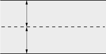
4.1 The matrix operator method 83
Level Optical depth
0
1
2
τ
0
τ
1
τ
2
(0, 1) = τ
1
− τ
0
(1, 2) = τ
2
− τ
1
Fig. 4.1 Subdivision of an inhomogeneous layer (0, 2) into two homogeneous
sublayers (0, 1) and (1, 2) having different optical properties.
(1, 2) = τ
2
− τ
1
. In general, however, the combined layer (0, 2) = τ
2
− τ
0
is inho-
mogeneous, see Figure 4.1.
For sublayer (0, 1) we will define the following optical quantities for the m-th
Fourier mode of the radiance which fully describe the transmission and reflection
properties.
t
m
(0, 1) discretized transmissivity (directions i = 1,...,s) of sublayer (0, 1)
applied to the radiance I
m
−
(τ
0
) incident at τ
0
,
t
m
(1, 0) discretized transmissivity for sublayer (1, 0) applied to the radiance I
m
+
(τ
1
)
incident at τ
1
,
r
m
(0, 1) discretized reflectivity (directions i = 1,...,s) of sublayer (0, 1) for the
radiance I
m
−
(τ
0
) incident at τ
0
,
r
m
(1, 0) discretized reflectivity for sublayer (1, 0) but for the radiance I
m
+
(τ
1
),
J
m
−,1
(0, 1) discretized source function for the downward directed primary scattered
sunlight generated in sublayer (0, 1),
J
m
+,1
(1, 0) discretized source function for the upward directed primary scattered
sunlight generated in sublayer (1, 0),
J
m
−,2
(0, 1) discretized source function for the downward thermal emission generated
in sublayer (0, 1),
J
m
+,2
(1, 0) discretized source function for the upward directed thermal emission
generated in sublayer (1, 0).
Similar definitions apply to the corresponding matrix and vector quantities for
sublayer (1, 2) and the combined layer (0, 2).
Let us consider Figure 4.2 describing the basic properties of the radiation model.
The radiation transmitted and reflected by an arbitrary layer depends linearly on
the incident radiation from above and below. This is the so-called linear interaction
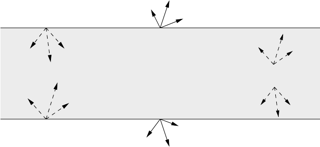
84 Quasi-exact solution methods for the RTE
I
m
()
I
m
+
()
I
m
+
−
−
−
−
()
J
m
+,1
(1, 0)
J
m
+,2
(1, 0)
J
m
,1
(0, 1)
J
m
,2
(0, 1)
Scattering
Absorption
Emission
τ
1
τ
1
τ
0
τ
1
I
m
()
τ
0
τ
0
Fig. 4.2 The linear interaction principle for the emanating radiation I
m
+
(τ
0
), I
m
−
(τ
1
)
from sublayer (0, 1) expressed in terms of the incident radiation I
m
+
(τ
1
), I
m
−
(τ
0
)
and the interior sources for primary scattering and thermal emission J
m
+,1
(1, 0),
J
m
+,2
(1, 0), J
m
−,1
(0, 1), J
m
−,2
(0, 1). In general, scattering, absorption and emission
take place.
principle. Therefore, the radiance emanating at τ
0
and τ
1
, expressed in terms of
the radiation I
m
−
(τ
0
), I
m
+
(τ
1
) incident at the boundaries of the sublayer (0, 1) and the
interior sources for primary scattering and thermal emission J
m
+,1
(1, 0), J
m
−,1
(0, 1),
J
m
+,2
(1, 0), J
m
−,2
(0, 1) is given by
(a) I
m
+
(τ
0
) = t
m
(1, 0)I
m
+
(τ
1
) + r
m
(0, 1)I
m
−
(τ
0
) + J
m
+,1
(1, 0) + J
m
+,2
(1, 0)
(b) I
m
−
(τ
1
) = r
m
(1, 0)I
m
+
(τ
1
) + t
m
(0, 1)I
m
−
(τ
0
) + J
m
−,1
(0, 1) + J
m
−,2
(0, 1)
(4.1)
In a similar manner we find for sublayer (1, 2)
(a) I
m
+
(τ
1
) = t
m
(2, 1)I
m
+
(τ
2
) + r
m
(1, 2)I
m
−
(τ
1
) + J
m
+,1
(2, 1) + J
m
+,2
(2, 1)
(b) I
m
−
(τ
2
) = r
m
(2, 1)I
m
+
(τ
2
) + t
m
(1, 2)I
m
−
(τ
1
) + J
m
−,1
(1, 2) + J
m
−,2
(1, 2)
(4.2)
If we replace in (4.1) the sublayer index 1 by index 2, we obtain for the combined
layer (0, 2) the result
(a) I
m
+
(τ
0
) = t
m
(2, 0)I
m
+
(τ
2
) + r
m
(0, 2)I
m
−
(τ
0
) + J
m
+,1
(2, 0) + J
m
+,2
(2, 0)
(b) I
m
−
(τ
2
) = r
m
(2, 0)I
m
+
(τ
2
) + t
m
(0, 2)I
m
−
(τ
0
) + J
m
−,1
(0, 2) + J
m
−,2
(0, 2)
(4.3)
It should be noted that in the last two equations the matrices t
m
(0, 2),
t
m
(2, 0), r
m
(0, 2), r
m
(2, 0) as well as the source vectors J
m
−,1
(0, 2), J
m
−,2
(0, 2),
J
m
+,1
(2, 0), J
m
+,2
(2, 0) are still unknown. We will show, however, that for the