Yamaguchi H. Engineering Fluid Mechanics (Fluid Mechanics and Its Applications)
Подождите немного. Документ загружается.

7.3 Viscoelastic Fluid and Flow
Note that for simplicity asterisk * in Eqs. (7.3.117) and (7.3.118) is
dropped in the resultant finite difference equations of Eqs. (7.3.125) and
(7.3.126).
For given initial and boundary conditions, i.e. Eqs. (7.3.119) to
(7.3.122), repeated use of Eqs. (7.3.125) and (7.3.126) generates the nu-
merical solution at all interior grid points
i
r at time level 1k . That is,
incrementing
k for time and substituting the known values of
1ki
u
,
and
1ki,
W
into the right hand side of Eqs. (7.3.125) and (7.3.126) allows the
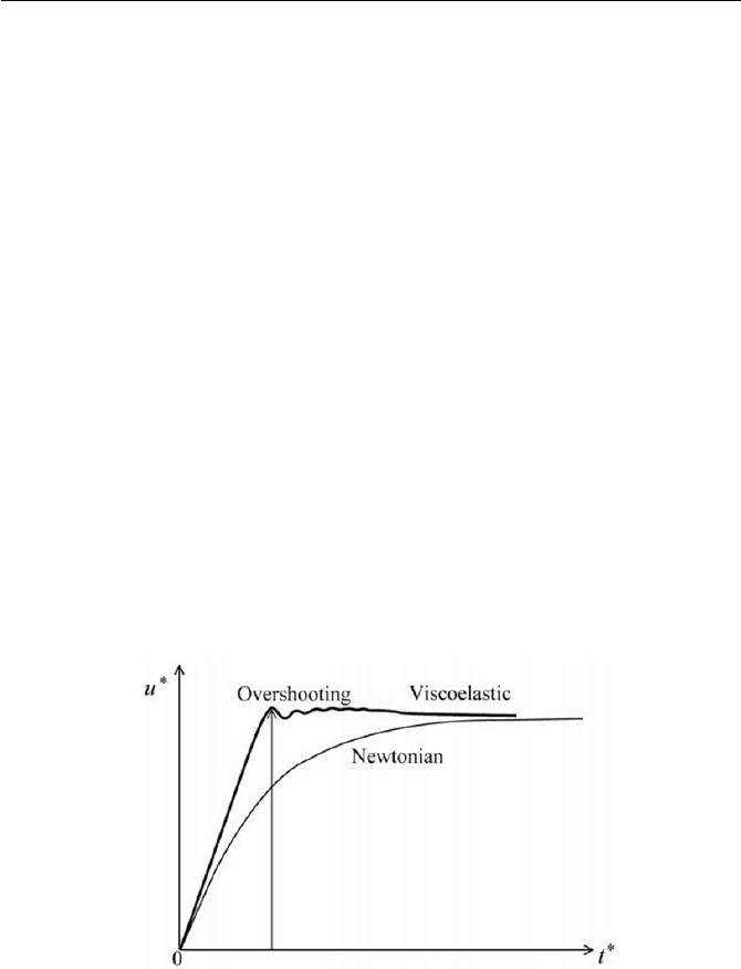
discrete solution to be marched toward in time. A typical numerical solu-
tion of
k
u
,1
, the time development of the axial velocity at the center of
pipe, is displayed in Fig. 7.22. As seen in the figure, an overshooting and
damping oscillation of the velocity are displayed for a step change of the
pressure gradient. It should be mentioned here that there might be some
difficulties for obtaining convergence of numerical solutions, depending
upon
]
and other geometric parameters.
art-up condition. Etter and Schowalter
(1965) calculated the transient behavior of viscoelastic flow of the same
problem, using Oldroyd-B model and showed similar overshooting charac-
ter of the flow parameter.
Fig. 7.22 Overshooting of flow parameter at start-up flow
The next important problem in viscoelastic fluid flow is the boundary
layer problem. In many engineering flow problems with viscoelastic fluids,
the pressure loss along the channel is a major concern, which is also di-
rectly connected with the formation of a boundary layer on the solid wall
of the channel. Let us examine the two dimensional boundary layer on a
flat plate (see Section 6.5.1 and refer Fig. 6.18). The effect of fluid elasticity
in viscoelastic fluid flow at sudden st
The overshooting of flow parameters is typically observed phenomena
475
7 Non-Newtonian Fluid and Flow
represented in the UCM equation of Eq. (7.3.47) can be included in the in-
tegral analysis of a boundary layer equation given in Eq. (6.5.33) by denot-
ing that the extra stress in an axial flow direction will introduce additional
terms inherited from the UCM equation. Denoting
b as the width of the
flat plate, the integral momentum equation at a steady state is written as
dyuUubxdxb
hx
w
³³
cc
00
UW
(7.3.127)
w
W
is the wall shear stress, u is the axial velocity in the boundary layer, U
is the velocity in the potential core and
h is the boundary thickness
G
th .
In the region
hy dd0 , a Maxwellian fluid is assumed to add the axial ex-
tra stress to the Newtonian wall shear stress
w
W
, so that Eq. ( 7.3.127) will
be newly written as
³³³
cc
hh
xx
x
w
dyuUubdyybxdxb
000
UWW
(7.3.128)
With regard to the axial extra stress contribution in Eq. (7.3.128),
xx
W
of
the UCM equation in simple shear flow is readily obtained from Eq.
(7.3.84) and it is
2
0
2
¸
¸
¹
·
¨
¨
©
§
w
w
y
u
xx
OKW
(7.3.129)
Substituting Eq. (7.3.129) for Eq. (7.3.128) and differentiating the equation
with respect to
x
yields
³
»
»
¼
º
«
«
¬
ª
¸
¸
¹
·
¨
¨
©
§
w
w
¸
¸
¹
·
¨
¨
©
§
w
w
h
w
dy
y
u
uUu
dx
d
y
u
0
2
2
OXX
(7.3.130)
where
U
K
X
0
is the kinematic viscosity. Therefore, as seen in Eq.
(7.3.130), the wall shear stress
w
w
yu ww
0
KW
is increased by the pres-
ence of elasticity. As in the Newtonian case, it is assumed that the similar-
ity of the velocity profiles is held at various sections along the boundary
layer development direction
x
. We can transform Eq. (7.3.130) into the
differential form for the boundary layer thickness
G
as follows
0
2
1
1
2
2
1
4
¸
¹
·
¨
©
§
Uc
c
dx
d
c
c
XG
G
OX
G
(7.3.131)
where
476
7.3 Viscoelastic Fluid and Flow
³
1
0
1
1
K
dffc ,
0
0
2
f
d
d f
c
c
¸
¸
¹
·
¨
¨
©
§
K
K
and
³
c
1
0
2
4
K
dfc
(7.3.132)
It is noted that
f and
K
are defined in Section 6.5, see Exercise 6.5.1, and
that
K
K
ff
n
. With the boundary condition
0
GG
at 0
x , Eq.
(7.3.132) is integrated to give
0ln21
2
0
4
2
0
2
0
12
¸
¹
·
¨
©
§
»
»
¼
º
«
«
¬
ª
¸
¹
·
¨
©
§
¸
¹
·
¨
©
§
G
G
OX
G
GGX
c
c
x
U
c
(7.3.133)
The root (
0
GG
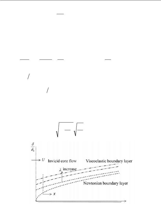
) in Eq. (7.3.133) would give us an insight on the phe-
nomenological explanation of the boundary layer development along a flat
plate, knowing that
0
GG
is a function of
x
, when implicitly calculated for
the variation of
x
. Figure 7.23 schematically shows the profiles of the vis-
coelastic and the Newtonian boundary layer. The boundary layer profile
for the viscoelastic flow tends, asymptotically, to Newtonian case at down-
stream, which is given as
U
x
c
c
x
X
G
¸
¹
·
¨
©
§
1
2
2
(7.3.134)
Fig. 7.23 Viscoelastic boundary layer
This is the same value as given in Eq. (6) in Exercise 6.5.1. As observed in
Fig. 7.23, the viscoelastic effect presented by adding the normal stress to
the Newtonian shear stress leads to the thickening of the boundary layer,
though giving a finite boundary layer thickness at the leading edge, i.e.
0
G
at
0 x .
477
7 Non-Newtonian Fluid and Flow
The physical interpretation of the thickening of the boundary layer may
be regarded as due to tensile stresses in the layer causing a thickening layer
while stretching the layer in an axial direction. At the leading edge, due to
a sudden thickening of the boundary layer formation, a finite value of
0
G
appears, which is, in effect, a purely hypothetical boundary condition in
terms of treating the problem via the constitutive equation.
Exercise
Display convective derivatives of the rate of a strain tensor for the simple
shear and shearfree flows at a steady state. Also show the relative strain
tensor for the simple shear and shearfree flows at a steady state. In like
manner obtain the convective derivatives of the stress tensors as well.
Consider the problems in Cartesian coordinates system.
Ans.
For the simple shear flow, we have relationships such that
ytyu
yxx
JJ
, 0
y
u and ,0
z
u considering that the steady state shear
rate
J
be constant. Similarly, for the shearfree flow, we can write relation-
ships such that
xtxu
xxx
HH
,
21 yktu
y
H
and
21 zktu
z
H
where
k is a constant 01 dd k , considering that the steady state elonga-
tional rate
H
be constant.
The rate of strain tensor for the simple shear flow is given via its com-
ponents
JJJ
¸
¸
¸
¹
·
¨
¨
¨
©
§
¸
¸
¸
¹
·
¨
¨
¨
©
§
¸
¸
¸
¹
·
¨
¨
¨
©
§
000
001
010
000
001
000
000
000
010
T
uuȖ
(1)
The upper convective derivative of the rate of stream tensor is written by
Exercise 7.3.1 Strains in Standard Flow
478
Exercise
222
22
000
000
001
2
000
000
001
2
000
000
001
2
000
001
010
000
001
000
000
001
010
000
001
010
000
000
010
000
001
010
JJJ
J
JJJ
¸
¸
¸
¹
·
¨
¨
¨
©
§
¸
¸
¸
¹
·
¨
¨
¨
©
§
¸
¸
¸
¹
·
¨
¨
¨
©
§
w
w
¸
¸
¸
¹
·
¨
¨
¨
©
§
¸
¸
¸
¹
·
¨
¨
¨
©
§
¸
¸
¸
¹
·
¨
¨
¨
©
§
¸
¸
¸
¹
·
¨
¨
¨
©
§
¸
¸
¸
¹
·
¨
¨
¨
©
§
¸
¸
¸
¹
·
¨
¨
¨
©
§
w
w
0
ȖȖȖ
t
t
Dt
D
T
uu
Ȗ
(2)
Note that higher order upper convective derivative
2tn is expressed by
)( n
and 0 is designated zero tensor (null tensor). Similarly, the corota-
tional convective derivative of the rate of strain tensor is expressed by
2
22
000
010
001
2
000
001
010
000
001
010
2
000
001
010
000
001
010
J
$
¸
¸
¸
¹
·
¨
¨
¨
©
§
¸
¸
¸
¹
·
¨
¨
¨
©
§
¸
¸
¸
¹
·
¨
¨
¨
©
§
¸
¸
¸
¹
·
¨
¨
¨
©
§
¸
¸
¸
¹
·
¨
¨
¨
©
§
ȖȖ
Dt
D
0
ȦȖȖȦ
Ȗ
Ȗ
(3)
The rate of strain tensor for the shearfree flow is similarly obtained
where
H
HH
¸
¸
¸
¹
·
¨
¨
¨
©
§
¸
¸
¸
¸
¸
¸
¹
·
¨
¨
¨
¨
¨
¨
©
§
¸
¸
¸
¸
¸
¸
¹
·
¨
¨
¨
¨
¨
¨
©
§
k
k
k
k
k
k
100
010
002
1
2
1
00
01
2
1
0
001
1
2
1
00
01
2
1
0
001
0Ȗ
(4)
and
479
7 Non-Newtonian Fluid and Flow
2
2
2
2
2
100
010
004
1
2
1
00
01
2
1
0
001
100
010
002
100
010
002
1
2
1
00
01
2
1
0
001
H
H
H
¸
¸
¸
¹
·
¨
¨
¨
©
§
¸
¸
¸
¸
¸
¸
¹
·
¨
¨
¨
¨
¨
¨
©
§
¸
¸
¸
¹
·
¨
¨
¨
©
§
¸
¸
¸
¹
·
¨
¨
¨
©
§
¸
¸
¸
¸
¸
¸
¹
·
¨
¨
¨
¨
¨
¨
©
§
k
k
k
k
k
k
k
k
k
k0Ȗ
(5)
0
00Ȗ
$
(6)
The relative strain tensor will be calculated by defining the displace-
ment functions
>@
tztytxt ,, r and
>@
tztytxt
c
ccccc
cc
,,r , when
we assume the simple shear flow equates to
yt
t
x
u
yxx
J
w
w
,
0
w
w
t
y
u
y
and
0
w
w
t
z
u
z
(7)
The displacement function
tt
cc
,r is written via the component form
yy
yxyttxtydtxx
yx
t
t
yx
c
c
cccc
c
³
c
JJJ
,
(8)
and
zz
c
(9)
The relative strain tensor
R
Ȗ
is written by definition, and which can be re-
duced to its component form likewise
I
,,
IEEICȖ
w
cc
w
w
cc
w
r
r
r
r
T
T
R
tttt
111
480
Exercise
¸
¸
¸
¹
·
¨
¨
¨
©
§
¸
¸
¸
¹
·
¨
¨
¨
©
§
¸
¸
¸
¹
·
¨
¨
¨
©
§
¸
¸
¸
¹
·
¨
¨
¨
©
§
000
00
0
100
010
001
100
01
001
100
010
01
2
J
JJ
J
J
(10)
In a similar fashion its inverse is given, where
¸
¸
¸
¹
·
¨
¨
¨
©
§
¸
¸
¸
¹
·
¨
¨
¨
©
§
¸
¸
¸
¹
·
¨
¨
¨
©
§
000
0
00
100
01
01
100
010
001
22
1
1
JJ
J
JJ
J
CICIȖ
R
(11)
Next, let us follow the same procedure where the relative strain tensors
are obtained for the shearfree flow by writing the velocity components as
xu
x
H
,
yku
y
1
2
H
and
zku
z
1
2
H
(12)
The displacement function
tt
cc
,r is written via its component form
x
tt
xxex
O
H
c
c
y
ktt
yyey
O
H
c
c
1
2
1
and
z
ktt
zzez
O
H
c
c
1
2
1
(13)
where
H
is the elongational strain defined as
³
c
cccc
c
t
t
tdttt
HH
,
(14)
This is called the Hencky strain. Thus, the relative strain tensors are ex-
pressed via the following forms
»
»
»
¼
º
«
«
«
¬
ª
100
010
001
2
2
2
1
z
y
x
R
O
O
O
ICȖ
(15)
and
481
7 Non-Newtonian Fluid and Flow
»
»
»
»
»
»
»
¼
º
«
«
«
«
«
«
«
¬
ª
2
2
2
1
100
0
1
10
00
1
1
z
y
x
R
O
O
O
CIȖ
(16)
Similarly the deviatoric stress tensors
IJ for the simple shear and uni-
axial stretching (shearfree) flows are written respectively
»
»
»
¼
º
«
«
«
¬
ª
zz
yyyx
xyxx
W
WW
WW
00
0
0
IJ
(17)
and
»
»
»
¼
º
«
«
«
¬
ª
zz
yy
xx
W
W
W
00
00
00
IJ
(18)
The upper convective and corotational derivatives are thus obtained for
dydu
x
xy
J
J
as follows
>@
T
Dt
D
uu
IJIJ
IJ
IJ
¸
¸
¸
¹
·
¨
¨
¨
©
§
¸
¸
¸
¹
·
¨
¨
¨
©
§
¸
¸
¸
¹
·
¨
¨
¨
©
§
¸
¸
¸
¹
·
¨
¨
¨
©
§
¸
¸
¸
¹
·
¨
¨
¨
©
§
¸
¸
¸
¹
·
¨
¨
¨
©
§
¸
¸
¸
¹
·
¨
¨
¨
©
§
000
00
02
000
00
00
000
000
0
00
0
001
000
00
0
0
00
0
0
000
000
010
yy
yyxy
yy
xyyyyx
zz
yyyx
xyxx
zz
yyyx
xyxx
IJ
IJIJ
IJ
IJIJIJ
IJ
IJIJ
IJIJ
IJ
IJIJ
IJIJ
JJJ
JJ
0
(19)
and
482
Exercise
(20)
000
0
2
0
2
000
001
010
00
0
0
2
00
0
0
000
001
010
2
¸
¸
¸
¸
¸
¸
¹
·
¨
¨
¨
¨
¨
¨
©
§
¸
¸
¸
¹
·
¨
¨
¨
©
§
¸
¸
¸
¹
·
¨
¨
¨
©
§
¸
¸
¸
¹
·
¨
¨
¨
©
§
¸
¸
¸
¹
·
¨
¨
¨
©
§
xy
yyxx
yyxx
xy
zz
yyyx
xyxx
zz
yyyx
xyxx
Dt
D
W
WW
WW
W
J
W
WW
WW
J
W
WW
WW
J
$
0
ȦIJIJȦ
IJ
IJ
Similarly setting the elongational rate at xu
xxx
ww
HH
for a shear-
free flow, where
H
is kept constant, the upper convective derivative and
the corotational derivative of
IJ are obtained respectively where
¸
¸
¸
¸
¸
¸
¹
·
¨
¨
¨
¨
¨
¨
©
§
¸
¸
¸
¸
¸
¸
¹
·
¨
¨
¨
¨
¨
¨
©
§
¸
¸
¸
¹
·
¨
¨
¨
©
§
¸
¸
¸
¹
·
¨
¨
¨
©
§
¸
¸
¸
¸
¸
¸
¹
·
¨
¨
¨
¨
¨
¨
©
§
zz
yy
xx
zz
yy
xx
zz
yy
xx
k
k
k
k
k
k
W
W
W
H
W
W
W
H
W
W
W
H
1
2
1
00
01
2
1
0
00
2
1
2
1
00
01
2
1
0
001
00
00
00
00
00
00
1
2
1
00
01
2
1
0
001
0IJ
(21)
and
000IJ
$
(22)
483
7 Non-Newtonian Fluid and Flow
Exercise 7.3.2 Integral UCM Equation in Standard Flow
Consider the integral UCM equation of Eq. (7.3.43), for the simple shear
flow and the shearfree flow at steady state. Give the rheological predic-
tions on the shear viscosity, the first normal stress difference, the second
normal stress difference and the elongational viscosity.
Ans.
The integral UCM equation is given via the following form, using the
relative strain tensor
>@
tdtte
tdtte
t
tt
t
R
tt
c
c
»
¼
º
«
¬
ª
cc
»
¼
º
«
¬
ª
³
³
f
c
f
c
1
2
0
2
0
I,C
,ȖIJ
O
O
O
K
O
K
(1)
where
1
C
is the Finger tensor. To obtain the shear viscosity
JWKK
xy
j ,
11
12
xy
CC component of the Finger tensor must be ob-
tained for the simple shear flow, namely, as it is exemplified in Exercise
7.3.1
tt
C
xyRxy
c
J
J
0
1
(2)
Therefore,
K
is computed where
0
2
0
1
K
J
O
K
JJ
W
K
O
cc
¸
¹
·
¨
©
§
c
f
³
tdtte
tt
t
xy
(3)
Thus, according to Eq. (3),
K
is kept constant for the variation of
J
. The
first normal stress difference
yyxx
N
WW
1
is obtained similarly when, in-
serting
tdttCC
yyxx
cc
2
211
J
, we have
2
0
11
2
0
1
2
JOK
O
K
WW
O
c
¸
¹
·
¨
©
§
c
f
³
tdCCeN
yyxx
tt
t
yyxx
(4)
484