Yamaguchi H. Engineering Fluid Mechanics (Fluid Mechanics and Its Applications)
Подождите немного. Документ загружается.


5.5 Oblique Shock Wave
E
tan
1
t
n
u
u
and
TE
tan
2
t
n
u
u
(5.5.6)
By defining
111
auM / , we can write
E
sin
111
Mau
n
/ since typically
E
sin
11
uu
n
. Thus, the normal shock relationship from Eq. (5.5.5) can be
written for the oblique shock relationship by replacing
1
M in Eq. (5.4.5)
with
E
sin
1
M , which gives
2sin1
sin1
22
1
22
1
1
2
2
1
E
E
U
U
Mk
Mk
u
u
n
n
(5.5.7)
Perhaps it is worth taking a moment to consider the relationship be-
tween the shock inclination angle
E
and the wedge angle
T
. Substituting
the relations from Eq. (5.5.6) into Eq. (5.5.7), we can derive the following
relationship between
E
and
T
E
E
E
TE
22
1
22
1
sin1
2sin1
tan
tan
Mk
Mk
(5.5.8)
By solving Eq. (5.5.8) for
T
, we can write the angle
T
as
E
E
E
T
cot
22cos
1sin2
tan
2
1
22
1
kM
M
(5.5.9)
Depending on
1
M , Eq. (5.5.9) shows that
T
will be zero for
E
, equal to
either
2
S
or
1
1
1sin M/
, or somewhere within this range, noting that
there is a maximum of
T
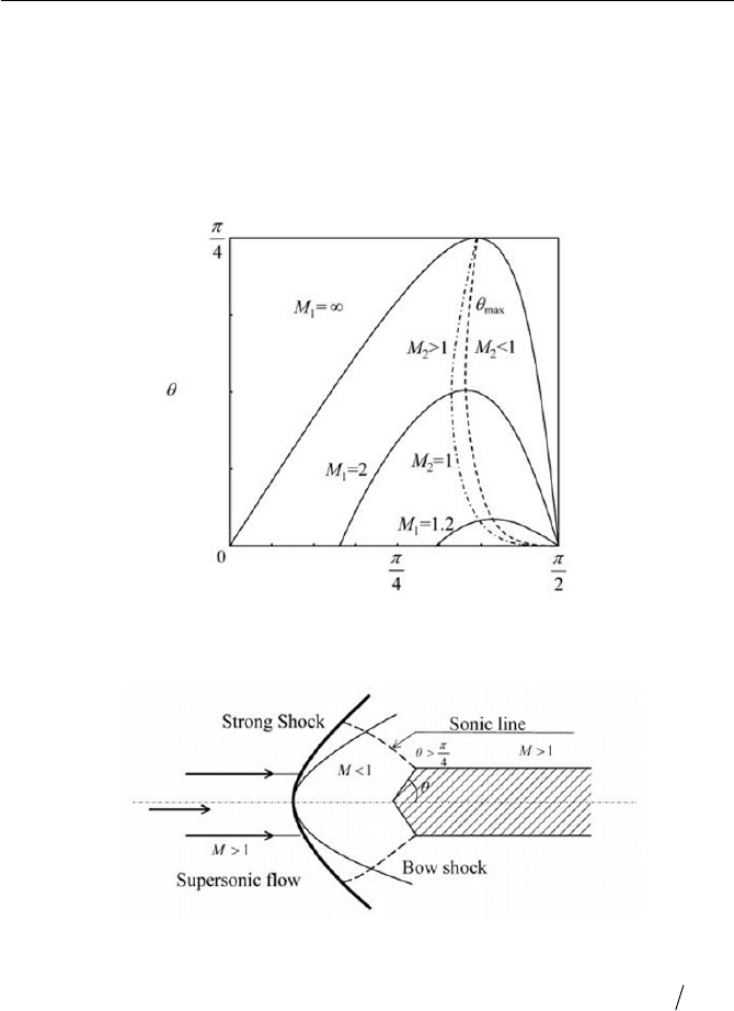
. Figure 5.12 is a plot of
T
versus
E
for a given
1
M , where the dashed line is a curve for max
T
. Figure 5.12 indicates that
there are two possible solutions of
E
for
T
4
S
T
. In practice it is ob-
served that the solution (to a weak shock) occurs and has a weaker discon-
tinuity, with a remainder of 1
2
!M (except for in a region between the
lines 1
2
M and
max
T
). That is, two solutions are derived from the jump
conditions, which are in effect characterized by different shock inclinations
angles and shock intensities. The solutions are known as the weak and
strong solutions. Phenomenologically the strong solution indicates a flow
which is subsonic downstream from the shock with
2
max
S
E
T
,
253
5 Compressible Flow
whereas the weak solution describes a flow which is supersonic down-
stream from the shock in
E
less than the line of 1
2
M . With a symmet-
rical slender wedge,
1
u is parallel to the surface of the wedge with an an-
gle of
T
, so that when
1
M is specified, the shock inclination angle
E
will
be calculated from Eq. (5.5.9).
Fig. 5.12
E
T
p
plot for an oblique shock
Fig. 5.13 Detached shock wave
It is interesting to see the flow phenomena if
T
is greater than
4ʌ
. It
appears that neither an oblique shock nor a normal shock is possible and it
is observed from experiment that the shock becomes detached. That is to
say, the shock curves around the wedge are not touching the wedge, as
schematically displayed in Fig. 5.13. The phenomenon also occurs with a
blunt body. There are some regions after the curved shock wave, called the
bow shock, as shown in Fig. 5.13. The dotted line, which corresponds to
254
Exercise
1
M
, is called the sonic line and divides the two regions of supersonic
and subsonic flow. It is found that the drag on a blunt body (or higher de-
flection angled wedge) is higher than that of a slender body when the body
is traveling with supersonic speed. This is due to the shock wave being de-
tached, and to reduce the drag it is advantageous to adopt a small nose an-
gle (wedge angle) for supersonic crafts so that the oblique shock may be
formed on the body.
Exercise
Exercise 5.1 The Compressibility Factor
In an isentropic flow through a channel from a reservoir, the pressure in
the reservoir is such that the velocity of flow is identically zero
㧚In con-
trast to the reservoir, when an isotropic flow is brought to rest at any point
of a flow field, the pressure with zero velocity can be obtained with the
same treatment as the case of a reservoir. The stagnation pressure is such
that a flow is brought to rest. We will now consider the stagnation pressure
0
p
for an isentropic flow in terms of the Mach number.
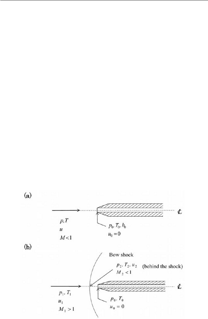
Fig. 5.14 The stagnation pressure; Pitot tube configuration
255
5 Compressible Flow
The typical application of such a flow is found by measuring its velocity
via the Pitot tube, as depicted in Fig. 5.14(a) and (b). Show the effect of
Mach number in measuring the stagnation pressure, and thus the velocity
of flow for an ideal gas.
Ans.
Let consider the energy equation of Eq. (5.2.13) between the upstream
and the stagnation, as indicated in Fig. 5.14(a)
hhuu
0
2
0
2
2
1
(1)
For an ideal gas we may write the enthalpy with the aid of the relations
Tch
p
and
00
Tch
p
. Also using
auM
and
1 kkRc
p
, we can
reduce Eq. (1) to the following form, by setting 0
0
ou
2
0
2
1
1
M
k
T
T
(2)
For the isentropic flow, we have a thermodynamic relation
1
00
¸
¸
¹
·
¨
¨
©
§
k
k
T
T
p
p
(3)
In combination with Eqs. (2) and (3), the stagnation pressure
0
p is thus
expressed by
1
2
0
2
1
1
¸
¹
·
¨
©
§
k
k
M
k
p
p
(4)
If this equation is expressed with a binomial expansion for the Mach num-
ber, we have
642
0
48
2
82
1
M
kk
M
k
M
k
p
p
(5)
and
¿
¾
½
¯
®
4
22
0
24
2
4
1
2
M
kMpkM
pp
(6)
It will prove useful to write the leading term of the right hand of Eq. (6) as
256
Exercise
22
2
2
2
1
2
1
22
uu
RT
p
kRT
u
k
ppkM
U
Thus, Eq. (6) becomes
c
M
kM
u
pp
D
U
4
2
2
0
24
2
4
1
2
1
(7)
The right hand side of Eq. (7) can be represented by
c
D
, which is called
the compressibility factor. For example, in the case of air
4.1 k
, it is cal-
culated that 2761
.
c
D
at 1
M
and in a lower Mach number case, we
can say that 0221
.
c
D
at 3.0 M . Thus, for measuring the velocity by a
Pitot tube, we can write the Eq. (7) as
2
1
0
2
c
pp
u
D
U
(8)
The actual velocity measured by a Pitot tube for a flow of 30
. M is ap-
proximately %1.1 less than that of incompressible flow measurement.
In supersonic flow, however, a detached shock wave may be formed
ahead of a Pitot tube as shown in Fig. 5.14(b). Along the center line, the re-
lationship across a normal shock can be applied that are found in Eqs.
(5.4.18) and (5.4.6), written as
12
21
2
1
2
1
2
2
kkM
Mk
M and
1
12
2
1
1
2
k
kkM
p
p
(9)
The isentropic relation of Eq. (4) can be used between the point of after
shock to the stagnation point as indicated in Fig. 5.14(b), which is given as
1
2
2
2
0
2
1
1
¸
¹
·
¨
©
§
k
k
M
k
p
p
(10)
With Eqs. (9) and (10), eliminating
2
M and
2
p , we can derive the follow-
ing relationship between the upstream and the stagnation point
257
5 Compressible Flow
1
1
2
1
1
2
1
0
12
1
2
°
°
°
¿
°
°
°
¾
½
°
°
°
¯
°
°
°
®
¸
¸
¹
·
¨
¨
©
§
k
k
k
kkM
k
M
p
p
(11)
Equation (11) relates the stagnation pressure for a supersonic flow and the
formula is called the Rayleigh’s Pitot-tube relation.
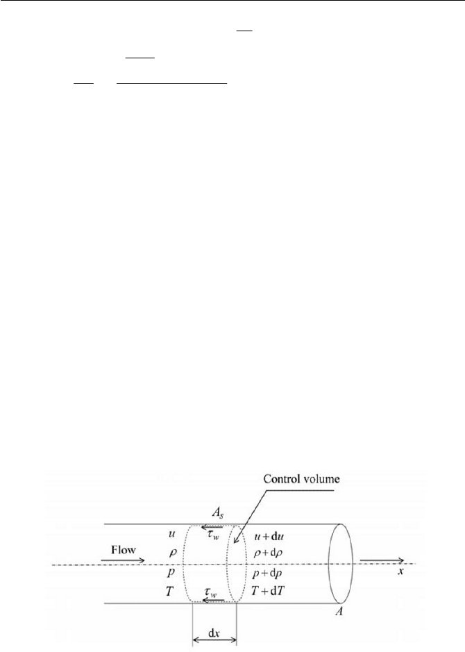
Exercise 5.2 Fanno-line Flow Relations and Chocking
Consider a flow of ideal gas in a horizontal tube of constant cross-section.
The flow in the tube is assumed adiabatic, but with friction, i.e. the exis-
tence of wall shear stress. Derive Fanno-line flow relations and discuss the
possibility of chocking condition.
Ans.
Let denote A as the cross-section area and dx as a small increment of
x
as indicated in Fig. 5.15, where the control volume is defined by dotted
line together with flow and thermodynamic parameters. For the control
volume, we will apply (i) the mass continuity, (ii) the momentum and (iii)
the energy equations as described below.
Fig. 5.15 Fanno-line flow,
w
W
t
the wall shear stress
258
Exercise
.const uA
U
(1)
For A constant, we can write Eq. (1) in a differential form as
0
u
dud
U
U
(2)
(ii) Momentum equation
The momentum balance of the control volume is
>@
sw
AAdpppAuduuuA
W
U
(3)
where
w
W
is the wall shear stress and
s
A
is the wall surface area of the
control volume.
w
W
can be defined, using the friction factor
f
c , as
¸
¹
·
¨
©
§
2
2
1
uc
fw
UW
(4)
We can assume that
f
c
is kept constant along the channel. It is reassuring
to know that the constant of
f
c is justified since it is kept around
00300040
.~.
f
c for the Reynolds number
69
1010 ~ , although
f
c is a
function of the Reynolds number, the Mach number and surface roughness
H
(RMS) of tube wall,
DRecc
ff
H
,, M . In a case of circular tube of
diameter
D
, i.e.
DdxA
s
S
, Eq. (1) can be rearranged as follows
0
4
2
1
2
¸
¹
·
¨
©
§
dx
D
c
p
dp
kM
u
du
f
(5)
where for
2222
kpMaMRTpu
U
is used and, a is the speed of
sound.
(iii) Energy equation
The energy equation of an ideal gas with the enthalpy defined as
Tch
p
is written from Eq. (5.2.13) as
0
dTcudu
p
(6)
By dividing the both sides by
Tc
p
and recognizing
1 kkRc
p
, we
can obtain
(i) Mass continuity equation
259
5 Compressible Flow
01
2
u
du
Mk
T
dT
(7)
It should be kept in mind that, as in Eqs. (1) to (7), there is no particular
thermodynamic process mentioned for the control volume, but with the
adiabatic condition to the control volume being assumed, we can assume
there is no heat transfer to or from the control volume.
(iv) Entropy change and Mach number
The equation of state for an ideal gas is written as
RTp
U
, and it’s
differential form is
T
dTd
p
dp
U
U
(8)
The entropy change of the control volume is, from the second law of ther-
modynamics
U
U
d
R
T
dT
cds
v
U
U
d
R
T
dT
k
R
1
(9)
It is noted again that the adiabatic condition to the control volume does not
directly mean it is isentropic, since we are considering the friction of flow.
From the definition of the Mach number
kRTuM , a differential form
is
T
dT
u
du
M
dM
2
1
(10)
Now we are able to reduce the Fanno-line of flow relations in terms of
the Mach number, using Eqs. (1) to (10). To begin with, eliminating
TdT
as in Eqs. (7) and (10) and by combining them with Eq. (2), we can obtain
U
U
d
dM
Mk
k
Mu
du
¿
¾
½
¯
®
2
22
21
11
2
1
(11)
Equation (11) is substituted into Eq. (7) and we have the relationship that
follows
260
Exercise
dM
Mk
Mk
MT
dT
¿
¾
½
¯
®
21
121
2
2
(12)
In the same manner, Eqs. (11) and (12) are substituted into Eq. (8) to give
dM
Mk
Mk
Mp
dp
¿
¾
½
¯
®
21
11
2
(13)
Thus, from the relationships derived from above, the entropy change is
given by substituting Eqs. (11) and (12) into Eq. (9)
dM
Mk
Mk
MR
ds
¿
¾
½
¯
®
21
11
2
(14)
Similarly, the actual change of the Mach number itself will be given by
substituting Eqs. (11) and (13) to Eq. (5) to give
dM
Mk
Mk
k
k
Mk
k
MkD
dx
c
f
¿
¾
½
¯
®
¸
¹
·
¨
©
§
21
111112
4
23
(15)
Table 5.1 Change of properties in the Fanno-line flow
Property Subsonic flow
1
M
Supersonic flow
1!
M
s
M
u
U
T
p
Equations (11) to (15) give the change of properties,
u
,
U
,
T
,
p
,
s
and
M
. It will be convenient to verify the changes of a state by the Mach
number whether the flow is subsonic or supersonic. Table 5.1 shows the
summarized results. As seen in Table 5.1, for subsonic flow ( 1
M
), when
the Mach number increases, the change of the Mach number along the tube
will be
0!dxdM from Eq. (15), implying the fact that the effective cross
section area decreases. This effect concerns the effective increase of the
thickness of the boundary layer, since the flow includes the effect of vis-
cosity.
From Table 5.1, we also see that the frictional effects cause the fluid to
tend toward 1
M
for both initially subsonic and supersonic conditions.
261
5 Compressible Flow
This fact indicates, if a tube length is sufficiently long enough, that the
flow is choked off due to the friction. We may be able to integrate Eqs.
(11)~(15) between a reference point of flow to a point where the flow
reaches the Mach number, as schematically depicted in Fig. 5.16. For ex-
ample, if we integrate Eq. (15), we obtain
dM
Mk
M
Mk
dx
D
c
M
x
x
f
³³
¿
¾
½
¯
®
1
2
2
3
21
122
4
*
(16)
and
2
2
2
2
max
1
21
1
In
2
1
4
kM
M
Mk
Mk
k
k
L
D
c
f
¿
¾
½
¯
®
(17)
where we set
xxL
max
.
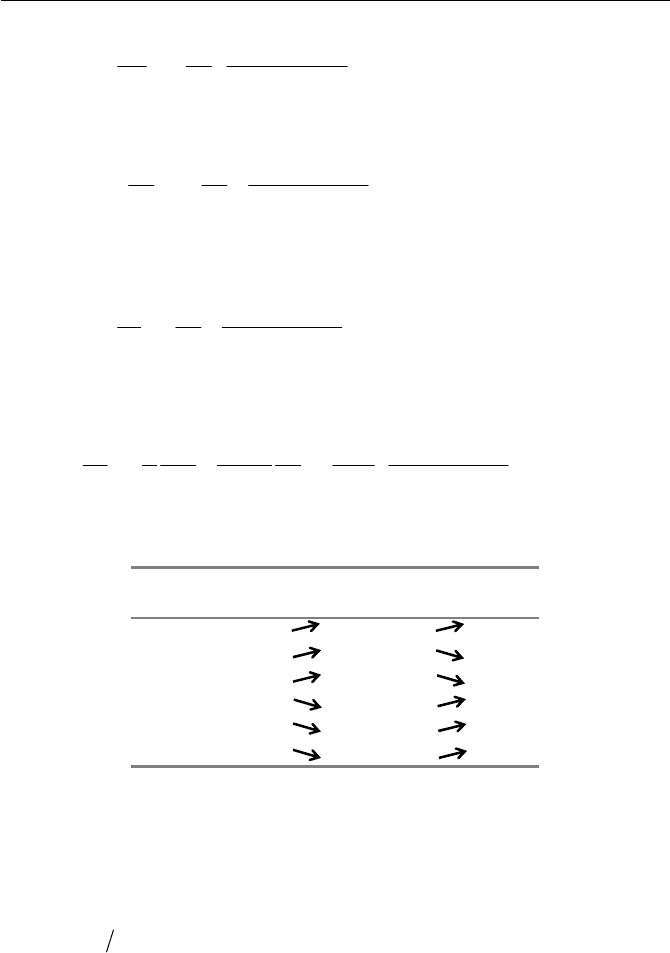
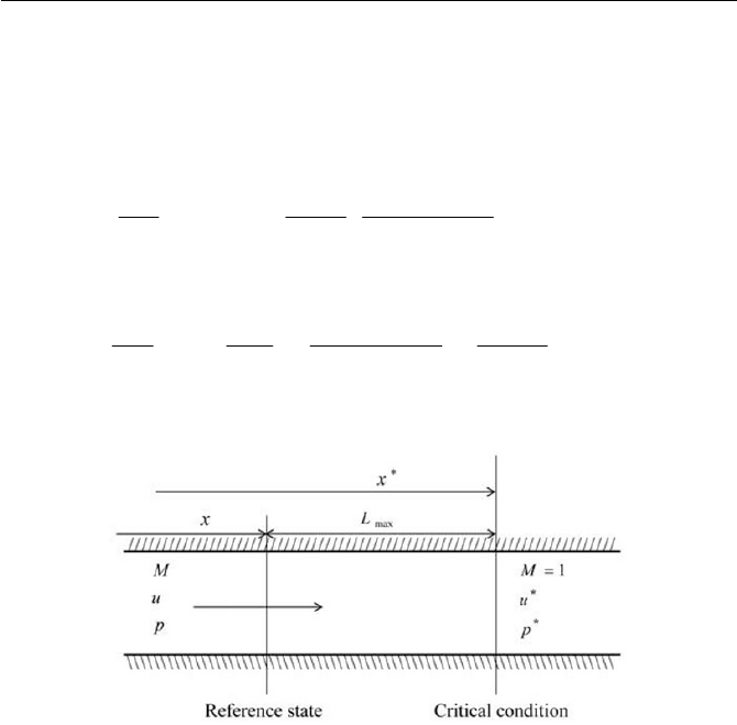
Fig. 5.16 Approach to critical condition
It appears that the flow reaches the choking condition at
*
xx from an ar-
bitrary point
x
in a tube.
max
L is the maximum length, which is called the
limiting length.
Now cases are examined in order to gain the trend in the properties
change along the distance, particularly in the Mach number. From Eq. (17),
Fig. 5.17 is a plot of a Mach number
2
M at a distance
2
x
from a refer-
ence point
x
, where a reference Mach number is denoted by
2
M . For ex-
ample, a flow with a Mach number 7.0
M at a point of
x
reaches
1
2
M at approximately 20
max2
. L where the flow is choked. In the case
where the length of tube is longer than
max2
L , the flow cannot reach 1
M
along the tube, but only at the exit, where the flow is chocked. The mass
flow rate decreases in the case of a tube longer than
max2
L . When a flow is
262