Warren J., Weimer H. Subdivision Methods for Geometric Design. A Constructive Approach
Подождите немного. Документ загружается.

64 CHAPTER 3 Convergence Analysis for Uniform Subdivision Schemes
Given a sequence of functions p
0
[x], p
1
[x], p
2
[x], ..., there are several ways to
define the limit of this sequence of functions. The simplest definition, pointwise
convergence, defines the limit
lim
k→∞
p
k
[x] = p
∞
[x] independently for each possible
value of
x.
The main drawback of pointwise convergence is that properties that are true
for a sequence of functions
p
k
[x] may not be true for their pointwise limit
p
∞
[x].For
example, consider the sequence of functions
p
k
[x] = x
k
. On the interval 0 ≤ x ≤ 1,
the limit function
p
∞
[x] is zero if x < 1 and one if x == 1. However, this function
p
∞
[x] is discontinuous, while for any k the monomial p
k
[x] is continuous. Thus, the
pointwise limit of a sequence of continuous functions is not necessarily a continuous
function.
Another drawback is that the derivatives of a sequence of functions
p
k
[x] do not
necessarily converge to the derivative of their pointwise limit. For example, consider
the piecewise linear function
p
k
[x] whose value at
i
2
k
is 2
−k
if i is odd and zero if i
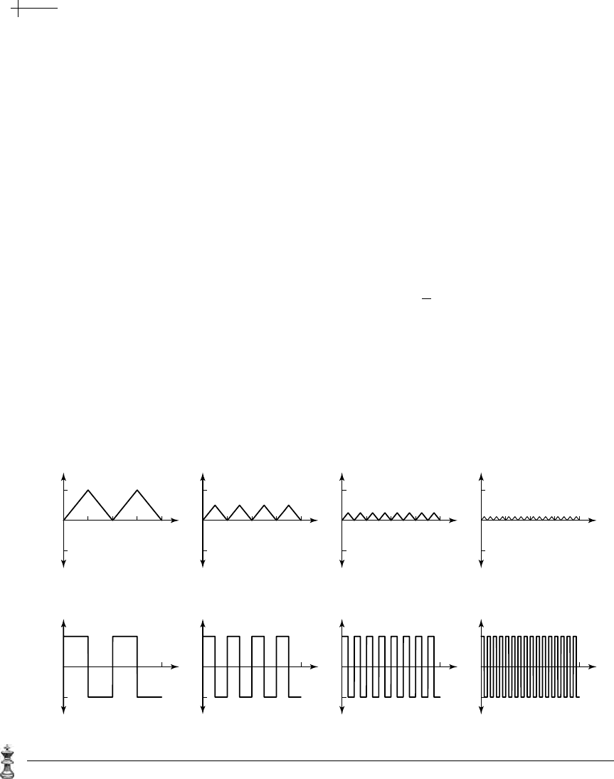
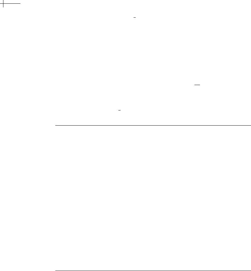
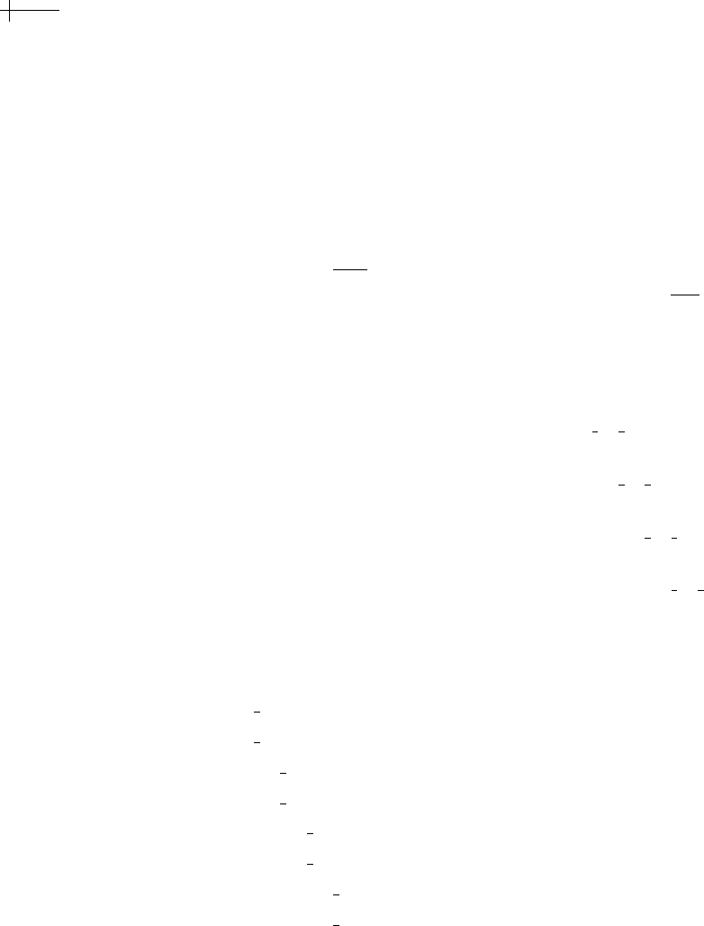
is even. The top portion of Figure 3.1 shows plots of these sawtooth functions for
k == 0, 1, 2, 3. Clearly, the pointwise limit of the functions p
k
[x] as k →∞is simply
the function zero. However, note that the derivative
p
k
[x] of these functions has
value
±1 for any value of k and does not converge to zero (i.e., the derivative of the
function zero) in any sense. The lower portion of Figure 3.1 shows plots of these
derivatives.
12 3
4
1
1
12 3
4
1
1
123
4
1
1
123
4
1
1
123
4
1
1
12 3
4
1
1
12 3
4
1
1
12 3
4
1
1
(a)
(b)
Figure 3.1 A sequence of functions converging to zero (a) whose derivatives (b) do not converge to zero.
3.1 Convergence of a Sequence of Functions 65
3.1.2 Uniform Convergence
The difficulties alluded to in the previous section lie in the definition of pointwise
convergence. Given an
, each value of x can have a distinct n associated with it
in the definition of pointwise convergence. A stronger definition would require
one value of
n that holds for all x simultaneously. To make this approach work, we
need a method for computing the difference of two functions over their entire
domain. To this end, we define the norm of a function
p[x], denoted by p[x],to
be the maximum of the absolute of
p[x] over all possible x; that is,
p[x]=Max
x
|p[x]|.
In standard numerical analysis terminology, this norm is the infinity norm of p[x].
(Observe that one needs to use care in applying this norm to functions defined on
infinite domains, because
Max is not always well defined for some functions, such
as
p[x] = x.) Based on this norm, we define a new, stronger type of convergence for
sequences of functions. A sequence of functions
p
k
[x] uniformly converges to a limit
function
p
∞
[x] if for all
>0 there exists an n such that for all k ≥ n
p
∞
[x] − p
k
[x] <.
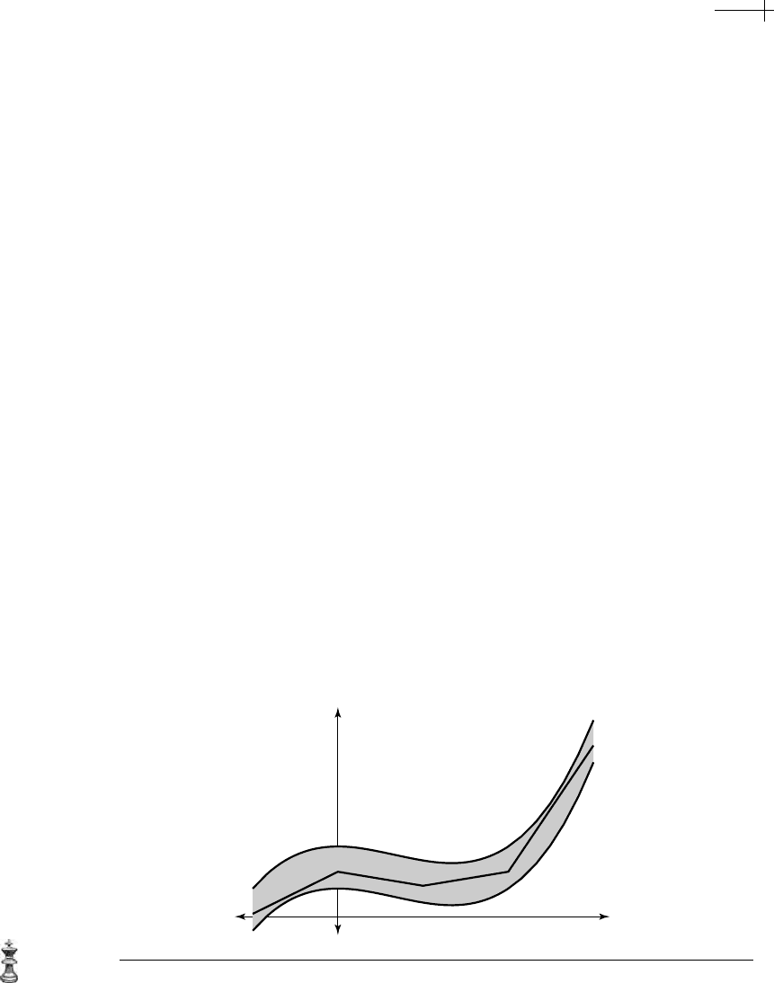
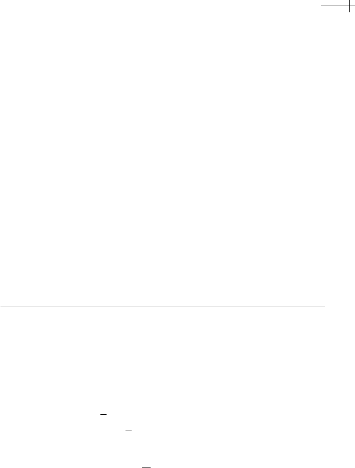
Figure 3.2 illustrates this definition. For k ≥ n, each function p
k
[x] must lie in the
ribbon bounded above by
p
∞
[x] + and bounded below by
p
∞
[x] − .
When proving that a sequence of functions
p
k
[x] defined by subdivision con-
verges uniformly to a limit function
p
∞
[x], we usually do not have access to the limit
ᒍ
ᒍ
ᒍ
k
Figure 3.2 Two functions p
∞
[x] ± bounding the function p
k
[x] in the definition of uniform convergence.
66 CHAPTER 3 Convergence Analysis for Uniform Subdivision Schemes
function p
∞
[x] beforehand. Thus, it is difficult to bound the norm p
∞
[x] − p
k
[x]
directly. Instead, we examine the norm of differences between successive approx-
imations
p
k
[x] − p
k−1
[x]. The following theorem establishes a useful condition
on these differences that is sufficient to guarantee uniform convergence of the
sequence of functions
p
k
[x].
THEOREM
3.1
Given a sequence of functions p
0
[x], p
1
[x], p
2
[x], ..., if there exist constants
0 <α<1 and β>0 such that
p
k
[x] − p
k−1
[x] <βα
k−1
for all k > 0, the sequence converges uniformly to a limit function p
∞
[x].
Proof To begin, we prove that there exists a pointwise limit p
∞
[x] for the functions
p
k
[x]. For a fixed value of x, we observe that the sum of the absolute value
of the difference of successive functions satisfies the inequality
k
j =1
|p
j
[x] − p
j −1
[x]| <
k
j =1
βα
j −1
== β
1 − α
k
1 − α
.
Because 0 <α<1, the expression β
1−α
k
1−α
converges to
β
1−α
as k →∞. There-
fore, by the comparison test (Theorem II, page 548 in [151]), the sum
∞
j =1
|p
j
[x] − p
j −1
[x]| is also convergent. Moreover, because this sum of ab-
solute values is convergent, the sum
∞
j =1
( p
j
[x]−p
j −1
[x]) is also convergent
(Theorem IX, page 557 in [151]). Given this convergence, we define the
pointwise limit of the subdivision process to be the infinite sum
p
∞
[x] == p
0
[x] +
∞
j =1
( p
j
[x] − p
j −1
[x]).
To conclude the proof, we prove that the functions p
k
[x] uniformly converge
to
p
∞
[x]. To this end, we observe that the difference p
∞
[x] − p
k
[x] can be
expressed as an infinite sum of the form
p
∞
[x] − p
k
[x] ==
∞
j =k+1
( p
j
[x] − p
j −1
[x]).
3.1 Convergence of a Sequence of Functions 67
Taking the norm of both sides of this expression and applying the triangle
inequality yields
p
∞
[x] − p
k
[x]≤
∞
j =k+1
p
j
[x] − p
j −1
[x].
Now, by hypothesis, the norm p
j
[x] − p
j −1
[x] is bounded by βα
k−1
. Sub-
stituting this bound into the infinite sum above yields
p
∞
[x] − p
k
[x]≤β
α
k
1 − α
.
Given an >0 from the definition of uniform continuity, we simply choose
k sufficiently large such that the right-hand side of this equation is less
than
. This condition ensures that the functions p
k
[x] converge uniformly
to
p
∞
[x].
3.1.3 Uniform Convergence for Continuous Functions
One advantage of uniform convergence over pointwise convergence is that it guar-
antees that many important properties of the functions
p
k
[x] also hold for the limit
function
p
∞
[x]. In the case of subdivision, the most important property is conti-
nuity. By construction, the piecewise linear approximations
p
k
[x] are continuous.
Thus, a natural question to ask is whether their limit
p
∞
[x] is also continuous. If
the convergence is uniform, the answer is yes. The following theorem establishes
this fact.
THEOREM
3.2
Let p
k
[x] be a sequence of continuous functions. If the sequence p
k
[x] con-
verges uniformly to a limit function
p
∞
[x], then p
∞
[x] is continuous.
Proof We begin by recalling the definition of continuity for a function. The func-
tion
p
∞
[x] is continuous at x = x
0
if given an >0 there exists a neighbor-
hood of
x
0
such that |p
∞
[x] − p
∞
[x
0
]| <for all x in this neighborhood. To
arrive at this inequality, we first note that due to the uniform convergence
of the
p
k
[x], for any >0 there exists an n independent of x such that,
68 CHAPTER 3 Convergence Analysis for Uniform Subdivision Schemes
for all k ≥ n, |p
k
[x] − p
∞
[x]| <
3
for all x. At this point, we can expand the
expression
p
∞
[x] − p
∞
[x
0
] in the following manner:
p
∞
[x] − p
∞
[x
0
] == ( p
∞
[x] − p
k
[x]) + ( p
k
[x] − p
k
[x
0
]) + ( p
k
[x
0
] − p
∞
[x
0
]),
|p
∞
[x] − p
∞
[x
0
]|≤|p
∞
[x] − p
k
[x]|+|p
k
[x] − p
k
[x
0
]|+|p
k
[x
0
] − p
∞
[x
0
]|.
Combining these two inequalities yields a new inequality of the form
|p
∞
[x] − p
∞
[x
0
]| < |p
k
[x] − p
k
[x
0
]|+
2
3
.
Because p
k
[x] is continuous at x
0
, there exists a neighborhood of x
0
for
which
|p
k
[x] − p
k
[x
0
]| <
3
holds. Thus, |p
∞
[x] − p
∞
[x
0
]| < for all x in this
neighborhood of
x
0
.
One immediate consequence of this theorem is that anytime we prove that the
piecewise linear approximations
p
k
[x] for a subdivision scheme converge uniformly
the resulting limit function
p
∞
[x] is automatically continuous.
3.1.4 Uniform Convergence for Smooth Functions
As we saw earlier in this section, one drawback of pointwise convergence is that it
does not ensure that the derivative of the functions
p
k
[x] converge to the derivative
of the limit function
p
∞
[x]. Because the derivatives p
k
[x] of the piecewise linear
functions
p
k
[x] associated with a subdivision scheme are piecewise constant func-
tions, we arrive at another natural question: Do these piecewise constant functions
p
k
[x] converge to the derivative of p
∞
[x] (i.e., of the limit of the functions p
k
[x])? The
answer is yes if the functions
p
k
[x] converge uniformly to a continuous function.
The following theorem is a slight variant of Theorem V, page 602 in [151].
THEOREM
3.3
Let the functions p
k
[x] converge uniformly to p
∞
[x]. If the derivative func-
tions
p
k
[x] converge uniformly to a function q[x], then q[x] is the derivative
of
p
∞
[x] with respect to x.
Proof We start by showing that
x
0
p
k
[t] dt is pointwise convergent to
x
0
q[t] dt for
all
x. Given that the functions p
k
[x] converge uniformly to q[x] as k →∞,
for all
>0 there exists n such that for all k ≥ n
|p
k
[t] − q[t]| <
3.2 Analysis of Univariate Schemes 69
for all t. For a fixed x , integrating the left-hand side of this expression on
the range
[0, x] yields
x
0
( p
k
[t] − q[t])
dt
≤
x
0
|p
k
[t] − q[t]|
dt ≤ x
for all k ≥ n. Recalling that p
k
[t] is by definition the derivative of p
k
[t], the
left-hand side of this expression reduces to
p
k
[x] − p
k
[0] −
x
0
q[t] dt
≤ x.
Given a fixed x, this inequality implies that the limit of
p
k
[x] − p
k
[0] as
k →∞is exactly
x
0
q[t] dt. However, by assumption, p
k
[x] − p
k
[0] also con-
verges to
p
∞
[x] − p
∞
[0]. Therefore,
p
∞
[x] ==
x
0
q[t] dt + p
∞
[0]
for any choice of x. Thus, q[x] is the derivative of p
∞
[x] with respect to x.
3.2 Analysis of Univariate Schemes
The univariate subdivision schemes considered in the previous chapter generated a
sequence of vectors
p
k
via the subdivision relation p
k
[x] = s[x ]p
k−1
[x
2
]. Associating
each vector
p
k
with a grid
1
2
k
Z yields a sequence of piecewise linear functions p
k
[x]
whose value at the i th knot, p
k
$
i
2
k
%
,isthe
i th entry of the vector p
k
; that is,
p
$
i
2
k
%
= p
k
[[ i ]] .
This section addresses two main questions concerning the sequence of functions
produced by this subdivision scheme: Does this sequence of functions
p
k
[x] con-
verge uniformly to a limit function
p
∞
[x]? If so, is this limit function smooth? The
answers to these questions have been addressed in a number of papers, including
those by Dahmen, Caveretta, and Micchelli in [17] and Dyn, Gregory, and Levin
in [51]. An excellent summary of these results appears in Dyn [49].
70 CHAPTER 3 Convergence Analysis for Uniform Subdivision Schemes
3.2.1 A Subdivision Scheme for Differences
To answer the first question, we begin with the following observation: If the max-
imal difference between consecutive coefficients of
p
k
goes to zero as k →∞, the
functions
p
k
[x] converge to a continuous function. If d[x] is the difference mask
(1 − x), the differences between consecutive coefficients of p
k
are simply the co-
efficients of the generating function
d[x]p
k
[x]. Intuitively, as the coefficients of
d[x]p
k
[x] converge to zero, any jumps in the associated linear functions p
k
[x] be-
come smaller and smaller. Therefore, the functions
p
k
[x] converge to a continuous
function
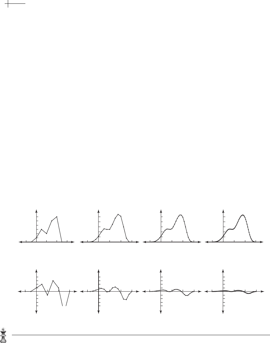
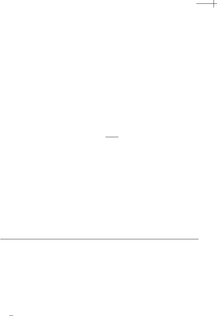
p[x]. Figure 3.3 shows plots of these differences for three rounds of cubic
B-spline subdivision. Note that the maximum value of these differences is decreas-
ing geometrically.
Our task in this and the next section is to develop a method for explicitly
bounding the decay of these differences in terms of the subdivision mask
s[x ].At
the heart of this method is the observation that if two consecutive approximations
p
k−1
[x] and p
k
[x] are related by the subdivision mask s[x] (by p
k
[x] = s[x ] p
k−1
[x
2
])
then the differences at consecutive levels,
d[x]p
k−1
[x] and d[ x]p
k
[x], are themselves
also related by a subdivision mask
t[x ]:
d[x]p
k
[x] == t[x ](d[x
2
]p
k−1
[x
2
]). (3.1)
2
2
4
6
4
3
2
1
1
2
3
4
2
24 6
4
3
2
1
1
2
3
4
2
24 6
4
3
2
1
1
2
3
4
2
24 6
4
3
2
1
1
2
3
4
22
4
6
1
2
3
4
5
6
22
4
6
1
2
3
4
5
22
4
6
1
2
3
4
5
2
2
4
6
1
2
3
4
5
(a)
(b)
Figure 3.3 Three rounds of cubic B-spline subdivision (a) and corresponding differences (b).
3.2 Analysis of Univariate Schemes 71
Under a relatively mild assumption concerning the structure of s[x], this new
subdivision mask
t[x ] can be constructed directly from s[x]. If we assume that the
subdivision process defined by
s[x ] is invariant under affine transformations, the
rows of the associated subdivision matrix
S must sum to one. For uniform subdi-
vision schemes, the matrix
S has two types of rows: those corresponding to the
odd-indexed coefficients
s[[2i +1]]
of s[x] and those corresponding to even-indexed
coefficients
s[[2i ]] of s[x]. Requiring the rows of S to sum to one is equivalent to
requiring each of these coefficient sequences to sum to one. Using simple linear
algebra, this condition can be expressed directly in terms of the mask
s[x ] as s[1] == 2
and s[−1] == 0. Under the assumption that s[−1] == 0, the following theorem (cred-
ited to Dyn, Gregory, and Levin [51]) relates the masks
s[x ] and t[x].
THEOREM
3.4
Given a subdivision mask s[x ] satisfying s[−1] == 0, there exists a subdivi-
sion mask
t[x ] relating the differences d[x]p
k−1
[x] and d[ x]p
k
[x] of the form
t[x ] =
s[x ]
1 + x
.
Proof Recall that the approximations p
k−1
[x] and p
k
[x] are related via p
k
[x] =
s[x ] p
k−1
[x
2
]. Multiplying both sides of this expression by the difference
mask
d[x] yields
d[x]p
k
[x] == d[x] s[x]p
k−1
[x
2
].
Because s[x] has a root at x == −1, the polynomial 1+x exactly divides s[x].
Therefore, there exists a mask
t[x ] satisfying the relation
d[x] s[x] == t[x ] d[x
2
]. (3.2)
Substituting the t[x ] d[x
2
] for d[x]s[x] in the previous equation yields
equation 3.1, the subdivision relation for the differences
d[x] p
k−1
[x] and
d[x] p
k
[x].
Note that equation 3.2 is at the heart of this theorem. One way to better un-
derstand this equation is to construct the associated matrix version of it. The matrix
analog
D of the difference mask d[x] = 1 − x is the bi-infinite two-banded matrix
with
−1 and 1 along the bands. If S and T are the bi-infinite two-slanted subdivision
72 CHAPTER 3 Convergence Analysis for Uniform Subdivision Schemes
matrices whose {i, j }-th entries are s[[i − 2j]] and t[[i − 2j]], respectively, the matrix
analog of equation 3.2 has the form
DS == TD. (3.3)
Note that the action of the difference mask d[x] in equation 3.2 is modeled by
multiplying the two-slanted matrix
S on the left by D, whereas the action of
the mask
d[x
2
] is modeled by multiplying the two-slanted matrix T on the right
by
D.
For example, if
s[x ] =
(1+x)
2
2x
, then s[x] is the subdivision mask for linear subdi-
vision. The subdivision mask
t[x ] for the difference scheme is simply
(1+x)
2x
.Inma-
trix form (showing only a small portion of the bi-infinite matrices), equation 3.3
reduces to
⎛
⎜
⎜
⎜
⎜
⎜
⎜
⎜
⎜
⎜
⎜
⎜
⎜
⎜
⎜
⎜
⎝
...........
. −110000000.
. 0 −11000000.
. 00−1100000.
. 000−110000.
. 0000−11000.
. 00000−1100.
. 000000−110.
. 0000000−11.
...........
⎞
⎟
⎟
⎟
⎟
⎟
⎟
⎟
⎟
⎟
⎟
⎟
⎟
⎟
⎟
⎟
⎠
⎛
⎜
⎜
⎜
⎜
⎜
⎜
⎜
⎜
⎜
⎜
⎜
⎜
⎜
⎜
⎜
⎜
⎜
⎜
⎜
⎜
⎝
.......
. 10000.
.
1
2
1
2
000.
. 01000.
. 0
1
2
1
2
00.
. 00100.
. 00
1
2
1
2
0 .
. 00010.
. 000
1
2
1
2
.
. 00001.
.......
⎞
⎟
⎟
⎟
⎟
⎟
⎟
⎟
⎟
⎟
⎟
⎟
⎟
⎟
⎟
⎟
⎟
⎟
⎟
⎟
⎟
⎠
==
⎛
⎜
⎜
⎜
⎜
⎜
⎜
⎜
⎜
⎜
⎜
⎜
⎜
⎜
⎜
⎜
⎜
⎜
⎜
⎜
⎜
⎝
......
.
1
2
000.
.
1
2
000.
. 0
1
2
00.
. 0
1
2
00.
. 00
1
2
0 .
. 00
1
2
0 .
. 000
1
2
.
. 000
1
2
.
......
⎞
⎟
⎟
⎟
⎟
⎟
⎟
⎟
⎟
⎟
⎟
⎟
⎟
⎟
⎟
⎟
⎟
⎟
⎟
⎟
⎟
⎠
⎛
⎜
⎜
⎜
⎜
⎜
⎜
⎜
⎝
.......
. −11000.
. 0 −1100.
. 00−110.
. 000−11.
.......
⎞
⎟
⎟
⎟
⎟
⎟
⎟
⎟
⎠
.
3.2 Analysis of Univariate Schemes 73
3.2.2 A Condition for Uniform Convergence
Given Theorem 3.4, we are now ready to state a condition on the subdivision mask
t[x ] for the differences that is sufficient to guarantee that the associated piecewise
linear functions
p
k
[x] converge uniformly. This condition involves the size of the
various coefficients
t[[ i]] of this mask. To measure the size of this sequence of co-
efficients, we first define a vector norm that is analogous to the previous functional
norm. The norm of a vector
p has the form
p=Max
i
|p[[ i ]]|.
(Again, this norm is the infinity norm in standard numerical analysis terminology.)
Given this vector norm, we can define a similar norm for a matrix
A of the form
A=Max
p=0
Ap
p
.
Observe that if the matrix A is infinite it is possible that the infinite sum denoted
by the product
Ap is unbounded. However, as long as the matrix A has rows with
only a finite number of non-zero entries, this norm is well defined. One immediate
consequence of this definition of
A is the inequality Ap≤Ap for all column
vectors
p. We leave it as a simple exercise for the reader to show that the norm of
a matrix
A is the maximum over all rows in A of the sums of the absolute values in
that row (i.e.,
A=Max
i
j
|A[[i, j]]|). Using these norms, the following theorem
(again credited to Dyn, Gregory, and Levin [51]) characterizes those subdivision
schemes that are uniformly convergent.
THEOREM
3.5
Given an affinely invariant subdivision scheme with associated subdivision
matrix
S, let the matrix T be the subdivision matrix for the differences
(i.e.,
T satisfies DS == TD). If T < 1, the associated functions p
k
[x] con-
verge uniformly as
k →∞for all initial vectors p
0
with bounded norm.
Proof Our approach is to bound the difference between the functions p
k
[x] and
p
k−1
[x] and then apply Theorem 3.1. Because p
k−1
[x] is defined using piece-
wise linear interpolation, it interpolates the coefficients of
Sp
k−1
plotted
on
1
2
k
Z, where
S is the subdivision matrix for linear subdivision. Therefore,
p
k
[x] − p
k−1
[x] == p
k
−
Sp
k−1
. (3.4)