Voet D., Voet Ju.G. Biochemistry

Подождите немного. Документ загружается.

g. Group II Chaperonins Have Built-In Lids

Group II chaperonins structurally and functionally re-

semble Group I chaperonins but consist of back-to-back

rings of 8 or 9 subunits and have no corresponding cochap-

erones such as GroES. Archaeal Group II chaperonins,

which are called thermosomes, consist of 1 to 3 different

types of subunits. Eukaryotic Group II chaperonins, which

are named TRiC (for TCP-1 ring complex;TCP for T-com-

plex polypeptide) or alternatively CCT (for chaperonin-

containing TCP-1), have dual octameric rings, each consist-

ing of eight genetically distinct but homologous subunits

arranged in a specific order. Like GroEL/ES, each of the

TRiC subunits couple the hydrolysis of ATP to the folding

of substrate proteins. Around 10% of eukaryotic cytosolic

proteins transiently interact with TRiC, many of which

have an absolute requirement for TRiC-aided folding.

These include a variety of essential structural and regula-

tory proteins including the muscle proteins actin and

myosin (Section 35-3A), the major microtubule compo-

nents tubulins ␣ and ␤ (Section 35-3G), and proteins that

participate in signal transduction (Chapter 19) and cell cycle

regulation (Section 34-4D). The only characteristic that

these proteins appear to have in common is that they form

homo- or hetero-oligomeric complexes.

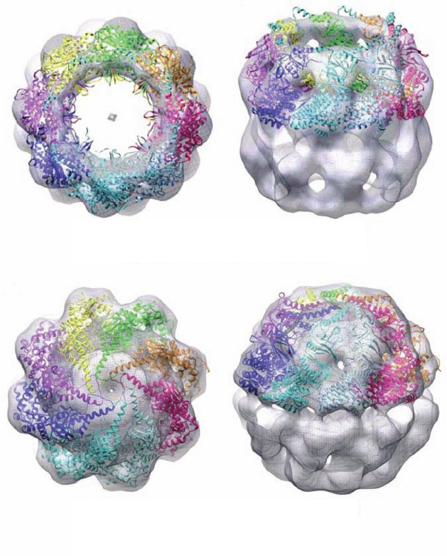
Cryo-electron microscopic (cryo-EM) studies of bovine

testes TRiC by Wah Chiu and Judith Frydman (Fig. 9-26)

revealed that, unlike GroEL, its overall shape is closer to

spherical than cylindrical. [In cryo-EM, the sample is

cooled to near liquid N

temperatures (⫺196°C) so rapidly

(in a few milliseconds) that the water in the sample does

not have time to crystallize but, rather, assumes a vitreous

(glasslike) state. Consequently, the sample remains hy-

drated and hence retains its native shape to a greater ex-

tent than in conventional electron microscopy (in which

the sample is vacuum dried).] Like GroEL,TriC’s subunits

each consist of equatorial, intermediate, and apical do-

mains. However, the tip of each TRiC apical domain has a

helical extension that GroEL lacks. TRiC has two confor-

mational states: an open state (Fig. 9-26a) in which each

helical extension is oriented more or less tangentially to

the inner portion of the ring, and a closed state (Fig. 9-26b)

in which each helical extension has swung to a more radial

Section 9-2. Folding Accessory Proteins 301

(a)

(b)

Top view

Open TRiC model versus EM open state

Side view

Top view

Closed TRiC model versus EM closed state

Side view

Figure 9-26 Structure of bovine testes

TRiC. (a) Its open state and (b) its closed

state. Surface diagrams of the cryo-EM-

based structures at ⬃16 Å resolution

(transparent gray) are shown as viewed

along the protein’s 8-fold axis (left) and as

viewed from the side with the 8-fold axis

tipped toward the viewer (right).The X-ray

structure of a homologous archaeal

chaperonin was modeled into the upper

ring of the cryo-EM-based image with each

subunit represented by a differently colored

ribbon diagram. [Courtesy of Judith

Frydman, Stanford University.]

JWCL281_c09_278-322.qxd 2/24/10 1:17 PM Page 301

orientation so as to form an iris-like lid that closes off the

TRiC cavity in a manner similar to the way that GroES

closes off the GroEL cavity. A lidless mutant of TRiC still

hydrolyzes ATP and binds unfolded actin with wild-type

affinity but is unable to induce its folding.This suggests that

the TRiC lid has a GroES-like function in coupling ATP

hydrolysis to the productive folding of substrate protein.

Interestingly, the putative substrate binding sites in TRiC

are not all hydrophobic as some of its subunits are lined

with polar residues. Perhaps each different substrate pro-

tein interacts with a specific combination of binding sites

on the apical domains in the open state of TRiC.

h. The Concept of Self-Assembly Must Take

Accessory Proteins into Account

Many proteins can fold/assemble to their native confor-

mations in the absence of accessory proteins, albeit often

with low efficiency. Moreover, accessory proteins are not

components of the native proteins whose folding/assembly

they facilitate. Hence, accessory proteins must mediate the

proper folding/assembly of a polypeptide to a conforma-

tion/complex governed solely by the polypeptide’s amino

acid sequence. Nevertheless, the concept that proteins are

self-assembling entities must be modified to incorporate

the effects of accessory proteins.

3 PROTEIN STRUCTURE PREDICTION

AND DESIGN

Since the primary structure of a protein specifies its three-

dimensional structure, it should be possible,at least in prin-

ciple, to predict the native structure of a protein from a

knowledge of only its amino acid sequence. This might be

done using theoretical methods based on physicochemical

principles, or by empirical methods in which predictive

schemes are distilled from the analyses of known protein

structures. Theoretical methods, which usually attempt to

determine the minimum energy conformation of a protein,

are mathematically quite sophisticated and require exten-

sive computations. The enormous difficulty in making such

calculations sufficiently accurate and yet computationally

tractable has, so far, limited their success. Nevertheless, an

understanding of how and why proteins fold to their native

structures must ultimately be based on such theoretical

methods. In this section we outline various methods that

have been used to predict the secondary and tertiary struc-

tures of proteins and end with a discussion of a related

technique, that of designing proteins that will have a partic-

ular structure.

A. Secondary Structure Prediction

The most reliable way to determine the secondary struc-

ture taken up by a polypeptide is to map its amino acid se-

quence onto that of a homolog of known structure. If, how-

ever, no such structure is available, the above-mentioned

predictive methods must be employed. Here we discuss the

use of empirical methods for secondary structure predic-

tion. The theoretical methods discussed in the following

section to predict a polypeptide’s tertiary structure will, of

necessity, also predict its secondary structure.

a. The Chou–Fasman Method

Empirical methods have had reasonable success in sec-

ondary structure prediction. Clearly, certain amino acid se-

quences limit the conformations available to a polypeptide

chain in an easily understood manner. For example, a Pro

residue cannot fit into the interior portions of a regular ␣ he-

lix or ␤ sheet because its pyrrolidine ring would fill the space

normally occupied by part of an abutting segment of chain

and because it lacks the backbone N¬H group with which

to contribute a hydrogen bond. Likewise, steric interactions

between several consecutive amino acid residues with side

chains branched at C

␤

(e.g., Ile and Thr) will destabilize an ␣

helix. Furthermore, there are more subtle effects that may

not be apparent without a detailed analysis of known pro-

tein structures. Here we shall discuss simple empirical meth-

ods for predicting the positions of ␣ helices, ␤ sheets, and re-

verse turns in proteins of known sequence.

The empirical structure prediction scheme developed

by Peter Chou and Gerald Fasman can be readily applied

by hand and is reasonably reliable. Its use requires two def-

initions. The frequency, f

␣

, with which a given residue oc-

curs in an ␣ helix in a set of protein structures is defined as

[9.3]f

␣

⫽

␣

302 Chapter 9. Protein Folding, Dynamics, and Structural Evolution

Table 9-1 Propensities and Classifications of Amino Acid

Residues for ␣ Helical and ␤ Sheet Conformations

Helix Sheet

Residue P

␣

Classification P

␤

Classification

Ala 1.42 H

␣

0.83 i

␤

Arg 0.98 i

␣

0.93 i

␤

Asn 0.67 b

␣

0.89 i

␤

Asp 1.01 I

␣

0.54 B

␤

Cys 0.70 i

␣

1.19 h

␤

Gln 1.11 h

␣

1.10 h

␤

Glu 1.51 H

␣

0.37 B

␤

Gly 0.57 B

␣

0.75 b

␤

His 1.00 I

␣

0.87 h

␤

Ile 1.08 h

␣

1.60 H

␤

Leu 1.21 H

␣

1.30 h

␤

Lys 1.16 h

␣

0.74 b

␤

Met 1.45 H

␣

1.05 h

␤

Phe 1.13 h

␣

1.38 h

␤

Pro 0.57 B

␣

0.55 B

␤

Ser 0.77 i

␣

0.75 b

␤

Thr 0.83 i

␣

1.19 h

␤

Trp 1.08 h

␣

1.37 h

␤

Tyr 0.69 b

␣

1.47 H

␤

Val 1.06 h

␣

1.70 H

␤

Source: Chou, P.Y. and Fasman, G.D., Annu. Rev. Biochem. 47, 258 (1978).

JWCL281_c09_278-322.qxd 2/24/10 1:17 PM Page 302

where n

␣

is the number of amino acid residues of the

given type that occur in ␣ helices and n is the total num-

ber of residues of this type in the set. The propensity of a

particular amino acid residue to occur in an ␣ helix is de-

fined as

[9.4]

where is the average value of f

␣

for all 20 residues.

Accordingly, a value of P

␣

⬎ 1 indicates that a residue oc-

curs with greater than average frequency in an ␣ helix. The

propensity, P

␤

, of a residue to occur in a ␤ sheet is similarly

defined.

Table 9-1 contains a list of ␣ and ␤ propensities based on

the analysis of 29 X-ray structures. In accordance with its

value of a given propensity, a residue is classified as a

strong former (H), former (h), weak former (I), indifferent

former (i), breaker (b), or strong breaker (B) of that sec-

ondary structure. Using these data, Chou and Fasman for-

mulated the following empirical rules (the Chou–Fasman

method) to predict the secondary structures of proteins:

␣

⫽

␣

1. A cluster of four helix-forming residues (H

␣

or h

␣

with I

␣

counting as one-half h

␣

) out of six contiguous

residues will nucleate a helix. The helix segment propa-

gates in both directions until the average value of P

␣

for a

tetrapeptide segment falls below 1.00. A Pro residue, how-

ever, can occur only at the N-terminus of an ␣ helix.

2. A cluster of three ␤ sheet formers (H

␤

or h

␤

) out of

five contiguous residues nucleates a sheet. The sheet is

propagated in both directions until the average value of P

␤

for a tetrapeptide segment falls below 1.00.

3. For regions containing both ␣- and ␤-forming se-

quences, the overlapping region is predicted to be helical if

its average value of P

␣

is greater than its average value of

␤

; otherwise a sheet conformation is assumed.

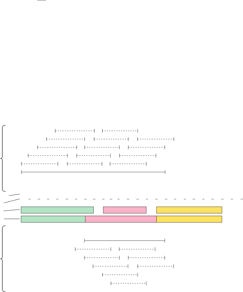
These easily applied empirical rules predict the ␣ helix and

␤ sheet strand positions in a protein with an average relia-

bility of ⬃50% and, in the most favorable cases, ⬃80%

(Fig. 9-27; note, however, that because proteins consist, on

average, of ⬃31% ␣ helix and ⬃28% ␤ sheet, random

predictions of these secondary structures would average

⬃30% correct).

Section 9-3. Protein Structure Prediction and Design 303

Figure 9-27 Secondary structure prediction. The prediction of

␣ helices and ␤ sheets was made by the Chou–Fasman method

and the prediction of reverse turns by the method of Rose for the

N-terminal 24 residues of adenylate kinase. The helix and sheet

propensities and classifications are taken from Table 9-1. The

solid lines indicate all hexapeptide sequences that can nucleate

an ␣ helix (top) and all pentapeptide sequences that can nucleate

a ␤ sheet (bottom), as is explained in the text. The average helix

and sheet propensities for each tetrapeptide segment in the helix

1.21

Met

Glu Glu

Lys

Leu

Lys Lys

Ser

Lys Ile Ile

Phe Val Val

Gly Gly

Pro

Gly Ser Gly

Lys

Gly

Thr

Gln

1.9 –3.5 –3.5 –3.9 3.8 –3.9 –3.9 –0.8 –3.9 4.5 4.5 2.8 4.2 4.2 –0.4 –0.4 –1.6 –0.4 –0.8 –0.4 –3.9 –0.4 –0.7 –3.5

1.05 0.37 0.37 0.74 1.30 0.74 0.74 0.75 0.74 1.60 1.60 1.38 1.70 1.70 0.75 0.75 0.55 0.75 0.75 0.75 0.74 0.75 1.19 1.10

1.45 1.51 1.51 1.16 1.16 0.77 1.16 1.08 1.08 1.13 1.06 1.06 0.57 0.57 0.57 0.77 0.57 1.16 0.57 0.83 1.11

Observed Helix Observed Sheet Observed Turn

Predicted Helix Predicted Sheet

1.41 1.06 1.08

1.35 1.04 0.96

1.26 1.02 0.82

1.17 1.11 0.69

1.08 1.09

0.96 1.38

1.17 1.22

0.941.33

1.57

1.60

α Helices

β Sheets

Hydropathy

Sequence

Observed

Predicted

1.16 0.57

Predicted Turn

and sheet regions are given above the corresponding dashed

lines.Twelve of the 15 residues are observed to have their

predicted secondary structures (middle), so that the prediction

accuracy, in this case, is 80%. Reverse turns are predicted to

occur in sequences in which the hydropathy (Table 8-6) is a

minimum and which do not occur in regions predicted to be

helical.The region that matches this criterion is observed to have

a reverse turn. [After Schultz, G.E. and Schirmer, R.H., Principles

of Protein Structure, p. 121, Springer-Verlag (1979).]

JWCL281_c09_278-322.qxd 2/24/10 1:17 PM Page 303

b. Reverse Turns Are Characterized by a Minimum

in Hydrophobicity Along a Polypeptide Chain

The positions of reverse turns can also be predicted by

the Chou–Fasman method. However, since a reverse turn

usually consists of four consecutive residues, each with a

different conformation (Section 8-1D), their prediction al-

gorithm is necessarily more cumbersome than those for

sheets and helices.

Rose has proposed a simpler empirical method for pre-

dicting the positions of reverse turns. Reverse turns nearly

always occur on the surface of a protein and, in part, define

that surface. Since the core of a protein consists of hy-

drophobic groups and its surface is relatively hydrophilic,

reverse turns occur at positions along a polypeptide chain

where the hydropathy (Table 8-6) is a minimum. Using

these criteria for partitioning a polypeptide chain, we can

deduce the positions of most reverse turns by inspection

(Fig. 9-27). Since this method often predicts reverse turns

to occur in helical regions (helices are all turns), it should

be applied only to regions that are not predicted to be

helical.

c. Physical Basis of ␣ Helix Propensity

Why do amino acid residues have such different

propensities for forming ␣ helices? This question has been

answered, in part, by Matthews through the structural and

thermodynamic analysis of T4 lysozyme (Section 9-1Bd) in

which Ser 44, a solvent-exposed residue in the middle of a

12-residue (3.3-turn) ␣ helix, was mutagenically replaced,

in turn, by all 19 other amino acids. The X-ray structures of

13 of these variant proteins revealed that, with the excep-

tion of Pro, the substitutions caused no significant distor-

tion to the ␣ helix backbone and, hence, that differences in

␣ helix propensities are unlikely to arise from strain. How-

ever, for 17 of the amino acids (all but Pro, Gly, and Ala),

the stability of the ␣ helix increases with the amount of side

chain hydrophobic surface that is buried (brought out of

contact with the solvent) when residue 44 is transferred

from a fully extended state to an ␣ helix. The low ␣ helix

propensity of Pro is due to the strain generated by its pres-

ence in an ␣ helix, and that of Gly arises from the entropic

cost associated with restricting this most conformationally

flexible of residues to an ␣ helical conformation (compare

Figs. 8-7 and 8-9) and its lack of hydrophobic stabilization.

The high ␣ helix propensity of Ala, however, is caused by

its lack of a ␥ substituent (possessed by all residues but Gly

and Ala) and hence the absence of the entropic cost associ-

ated with conformationally restricting such a group within

an ␣ helix together with its small amount of hydrophobic

stabilization.

d. Computer-Based Secondary Structure

Prediction Algorithms

A number of sophisticated computer-based secondary

structure prediction algorithms have been developed. Most

of them, like the Chou–Fasman method, employ sets of pa-

rameters whose values are determined by the analysis of

(learning from) a set of nonhomologous proteins with

known structures, in some cases coupled with energy mini-

mization techniques. These algorithms are typically ⬃60%

accurate in predicting which of three conformational

states, helix, sheet, or coil, a given residue in a protein

adopts. However, a significant increase in accuracy has

been gained (to over 80%) by employing evolutionary in-

formation through the use of multiple sequence align-

ments. This is because knowledge of the distribution of

residue identities at and around each position in a series of

homologous and presumably structurally similar proteins

provides a better indication of the protein’s structural ten-

dencies than does a single sequence.

Several secondary structure prediction algorithms are

freely available over the Web. Among them is Jpred3

(http://www.compbio.dundee.ac.uk/www-jpred/), which clas-

sifies residue conformations as being either helical (H),

extended/␤ sheet (E), or coil (⫺) with 81.5% reliability. It

requires as input either the sequence of a single polypep-

tide or a multiple sequence alignment. However, if Jpred3

is supplied with only a single sequence, it will first use PSI-

BLAST (Section 7-4Bi) to construct a multiple sequence

alignment.

Although we have seen that secondary structure is

mainly dictated by local sequences, we have also seen that

tertiary structure can influence secondary structure (Sec-

tion 9-1Be). The inability of sophisticated secondary struc-

ture prediction schemes to surpass ⬃80% reliability is

therefore partially explained by their failure to take terti-

ary interactions into account.

B. Tertiary Structure Prediction

The sequence databases (Section 7-4A) contain the sequences

of ⬃7 million polypeptides, and the rapid rate at which entire

genomes are being sequenced (Section 7-2C) promises that

many more such sequences will soon be known. Yet, only a

small fraction of the ⬃70,000 protein structures in the PDB

(Section 8-3B) are unique because many of them are of the

same protein binding different small molecules, mutant forms

of the same protein, or closely related proteins. Moreover,

around 40% of the open reading frames (ORFs; nucleic acid

sequences that appear to encode proteins) in known genome

sequences specify proteins whose function is unknown. Con-

sequently, formulating a method to reliably predict the native

structure of a polypeptide from only its sequence is a major

goal of biochemistry. In the following paragraphs we discuss

the progress that has been made in achieving this goal.

There are currently several major approaches to tertiary

structure prediction. The simplest and most reliable ap-

proach, comparative or homology modeling, aligns the se-

quence of interest with the sequences of one or more ho-

mologous proteins of known structure, compensating for

amino acid substitutions as well as insertions and deletions

(indels) through modeling and energy minimization calcu-

lations. For proteins with as little as 30% sequence identity,

this method can yield a root-mean-square deviation (rmsd)

between the predicted and observed positions of corre-

sponding C

␣

atoms of the “unknown” protein (once its

structure has been determined) of as little as ⬃2.0 Å. How-

ever, the accuracy of this method decreases precipitously

304 Chapter 9. Protein Folding, Dynamics, and Structural Evolution

JWCL281_c09_278-322.qxd 2/24/10 1:17 PM Page 304

(the rmsd’s rapidly increase) as the degree of sequence

identity drops below 30%. Conversely, for polypeptides

that are ⬎60% identical, a homology model may have

rmsd’s of ⬃1 Å (the accuracy of the atomic positions in an

⬃2.5-Å-resolution X-ray structure).

There are numerous instances of proteins that are struc-

turally similar even though their sequences have diverged

to such an extent that they have no apparent similarity.

Fold recognition or threading is a computational technique

that attempts to determine the unknown fold of a protein

by ascertaining whether its sequence is compatible with

any of the members of a library of known protein struc-

tures. It does so by placing the “unknown” protein’s

residues along the backbone of a known protein structure,

determining the stability of the side chains of the unknown

protein in that arrangement, and then sliding (threading)

the sequence of the unknown protein along that of the

known protein by one residue and repeating the calcula-

tion, etc., while allowing for the possibility of indels. If the

“correct” fold can be found (and there is no guarantee that

the fold of the unknown protein will resemble that of any

member of the library), the resulting model can be im-

proved via homology modeling. This method has yielded

encouraging results, although it cannot yet be considered

to be reliable. Of course, as sequence alignment algorithms

(Section 7-4B) improve in their ability to recognize distant

homologs, sequences that previously would have been can-

didates for fold recognition can instead be directly treated

by comparative modeling.

Since the native structure of a protein depends only on

its amino acid sequence, it should be possible, in principle,

to predict the structure of a protein based only on its

physicochemical properties (e.g., solvent interactions,

atomic volume, charge, hydrogen bonding properties, van

der Waals interactions, and bond torsion angle potentials

for all of its atoms). A major problem faced by such de

novo (Latin: from the beginning; synonymously ab initio)

methods is that polypeptide chains have astronomical

numbers of non-native low-energy conformations, so that it

requires extensive and highly detailed calculations to de-

termine a polypeptide’s lowest energy conformation.

To assess the effectiveness of the numerous de novo al-

gorithms that have been formulated, as well as other struc-

ture prediction schemes, a Critical Assessment of Structure

Prediction (CASP) has been held every 2 years starting in

1994. CASP participants are provided with the sequences

of proteins whose structures will soon be determined by

X-ray crystallography or NMR spectroscopy and submit

their predicted structures of these proteins for comparison

with the subsequently experimentally determined structures.

Over the years, de novo methods have steadily improved

from being little better than random guesses to predicting

the folding topologies of ⬍200-residue proteins with a suc-

cess rate of ⬃20% and occasionally with near-atomic accu-

racy. Rosetta, the most consistently successful de novo al-

gorithm in the past few CASPs, which was formulated by

David Baker, is enormously computer-intensive. To satisfy

its computational needs, Baker has organized a distributed

computer network known as Rosetta@home that uses the

otherwise idle time of nearly 100,000 volunteered comput-

ers so that an average of ⬃500,000 CPU-hours can be de-

voted to predicting the structure of each domain. Examples

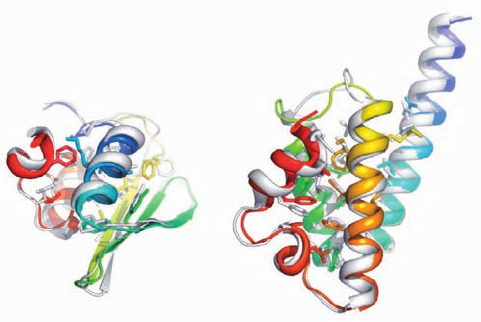
of successful protein structure predictions by Rosetta are

shown in Fig. 9-28.

C. Protein Design

Although we have not yet fully solved the protein folding

problem, considerable progress has been made in solving

the inverse problem: generating polypeptide sequences to

assume specific three-dimensional structures, that is, pro-

tein design. This is probably because a polypeptide can be

“overengineered” to take up a desired conformation. Con-

sequently, protein design has provided insights into protein

folding and stability, and it promises to yield useful pro-

teins that are “made to order.” Protein design begins with a

target structure such as a 4-helix bundle and attempts to

find an amino acid sequence that will form this structure.

The designed polypeptide is then synthesized and its struc-

ture elucidated.

Successful design requires not only that the desired fold

be stable but that other folds be significantly less stable (by

⬃15–40 kJ ⭈ mol

⫺1

). Otherwise a sequence that has been

found to be the most stable in the desired conformation

may actually be more stable in other conformations. Be-

fore such negative design concepts were implemented, ef-

forts to design proteins typically yielded an ensemble of

molten globulelike states rather than the desired folds.

Most successful protein design projects have redesigned

naturally occurring proteins so as to enhance their stability

or provide them with new functionalities. Because of the

Section 9-3. Protein Structure Prediction and Design 305

(a) (b)

Figure 9-28 Examples of successful modeling predictions by

Rosetta. Each panel shows the superposition of a predicted

model (gray) with the corresponding experimentally determined

X-ray structure colored in rainbow order from its N-terminus

(blue) to its C-terminus (red) with core side chains drawn as

sticks. (a) A protein of unknown function from Thermus

thermophilus HB8 (PDBid 1WHZ). The backbones are aligned

with an accuracy of 1.6 Å over 70 residues. (b) Protein BH3980

(10176605) from Bacillus halodurans (PDBid 2HH6).The

backbones are aligned with an accuracy of 1.4 Å over 90

residues. [Courtesy of Gautam Dantas, Washington University

School of Medicine.]

JWCL281_c09_278-322.qxd 2/24/10 1:17 PM Page 305

strict steric constraints in the cores of globular proteins,

this has largely yielded proteins whose internal side chain

packings resemble those of the original proteins. Conse-

quently, designing a protein with a novel fold should be a

more rigorous test of protein design methods. Indeed, it is

unlikely that a polypeptide of arbitrary sequence will have

a stable native structure.

Baker designed a topologically novel, 93-residue, ␣/␤

protein he named Top7 as follows. A rough two-dimen-

sional model of the target protein was created and struc-

tural constraints that defined its topology (e.g., hydrogen

bonds and reverse turns) were identified. Rosetta was then

used to generate 172 three-dimensional, backbone-only

models with the required topology by assembling 3- and 9-

residue fragments with the required secondary structures

from the Protein Data Bank (PDB). Side chains were ini-

tially placed by considering all sets of energetically allowed

torsion angles (which are known as rotamers) for each type

of side chain but Cys at the 71 core positions and for only

polar residues at the remaining 22 surface positions and us-

ing Rosetta to identify the lowest energy structures. These

models were then structurally optimized through 15 cycles

of using Rosetta to calculate the lowest energy backbone

conformation for a fixed amino acid sequence followed by

sequence redesign as previously described, ultimately

yielding Top7.Although the structural differences between

Top7 and its initial model were small (their backbones

have an rmsd of 1.1 Å), they had dramatic changes in se-

quence (with only 31% of the residues in Top7 being iden-

tical to those in its initial model).

A gene for Top7 with a C-terminal His tag was synthe-

sized (Section 7-6A) and expressed and the protein was pu-

rified by metal chelation affinity chromatography (Section

6-3Dg) followed by anion exchange chromatography (Sec-

tion 6-3A). Top7 is highly soluble in aqueous solution and

is monomeric as indicated by gel filtration chromatography

(Section 6-3B). It is remarkably stable: Its circular dichro-

ism (CD; Section 9-1Ca) spectrum at 98°C closely resem-

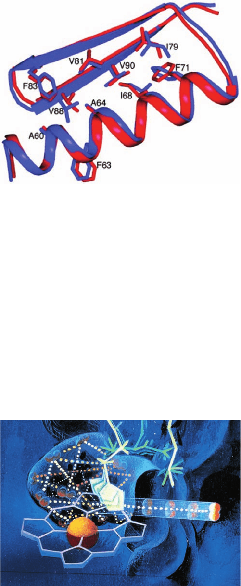
bles that at 25°C. The X-ray structure of Top7 is all but

identical, within experimental error, to the structure of the

designed model: Their rmsd over all backbone atoms is

1.17 Å and many of their core side chains are effectively su-

perimposable (Fig. 9-29). Evidently, protein folds that have

not been observed in nature are not only physically possi-

ble but can be highly stable.

Baker also used the principles of protein design to gen-

erate enzymes that catalyze nonbiological reactions. He did

so by grafting designed constellations of side chains onto

the surfaces of naturally occurring proteins so as to form

the desired active sites. As we shall see in Chapter 15, the

catalytic activities of enzymes are extraordinarily sensitive

to the positions of their catalytic groups.

4 PROTEIN DYNAMICS

The fact that X-ray studies yield time-averaged “snapshots”

of proteins may leave the false impression that proteins have

fixed and rigid structures. In fact, as is becoming increasing

clear, proteins are flexible and rapidly fluctuating molecules

whose structural mobilities have considerable functional sig-

nificance. For example, X-ray studies indicate that the heme

groups of myoglobin and hemoglobin are so surrounded by

protein that there is no clear path for O

to approach or es-

cape from its binding pocket. Yet we know that myoglobin

and hemoglobin readily bind and release O

. These proteins

must therefore undergo conformational fluctuations, breath-

ing motions, that permit O

reasonably free access to their

heme groups (Fig. 9-30). The three-dimensional structures of

myoglobin and hemoglobin undoubtedly evolved the flexi-

bility to facilitate the diffusion of O

to its binding pocket.

306 Chapter 9. Protein Folding, Dynamics, and Structural Evolution

Figure 9-29 Superposition of the designed model of Top7

(blue) with its X-ray structure (red). Core side chains are drawn

as sticks. [Courtesy of Gautam Dantas, Washington University

School of Medicine. PDBid 1QYS.]

Figure 9-30 Conformational fluctuations in myoglobin. An

artist’s conception of the “breathing” motions in myoglobin that

permit the escape of its bound O

molecule (double red spheres).

The dotted lines trace a trajectory an O

molecule might take in

worming its way through the rapidly fluctuating protein before

finally escaping. O

binding presumably resembles the reverse of

this process. [Illustration, Irving Geis. Image from the Irving

Geis Collection, Howard Hughes Medical Institute. Reprinted

with permission.]

JWCL281_c09_278-322.qxd 8/10/10 11:16 AM Page 306

The intramolecular motions of proteins have been clas-

sified into three broad categories according to their coher-

ence:

1. Atomic fluctuations, such as the vibrations of indi-

vidual bonds, which have time periods ranging from 10

⫺15

to 10

⫺11

s and spatial displacements between 0.01 and 1 Å.

2. Collective motions, in which groups of covalently

linked atoms, which vary in size from amino acid side

chains to entire domains, move as units with time periods

ranging from 10

⫺12

to 10

⫺3

s and spatial displacements be-

tween 0.01 and ⬎5 Å. Such motions may occur frequently

or infrequently compared with their characteristic time pe-

riod.

3. Triggered conformational changes, in which groups

of atoms varying in size from individual side chains to com-

plete subunits move in response to specific stimuli such as

the binding of a small molecule, for example,the binding of

ATP to GroEL (Section 9-2Ca). Triggered conformational

changes occur over time spans ranging from 10

⫺9

to 10

and result in atomic displacements between 0.5 and ⬎10 Å.

In this section, we discuss how these various motions are

characterized and their structural and functional signifi-

cance. We shall mainly be concerned with atomic fluctua-

tions and collective motions; triggered conformational

changes are considered in later chapters in connection with

specific proteins.

a. Proteins Have Mobile Structures

X-ray crystallographic analysis is a powerful technique

for the analysis of motion in proteins; it reveals not only the

average positions of the atoms in a crystal, but also their

mean-square displacements from those positions. X-ray

analysis indicates, for example, that myoglobin has a rigid

core surrounding its heme group and that the regions

toward the periphery of the molecule have a more mobile

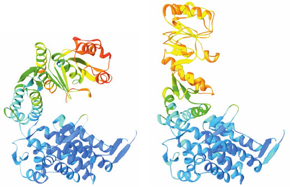
character. Similarly, the apical domain of GroEL and

the mobile loop of GroES are both highly flexible in the

individual proteins, but when they interact in the

GroEL–GroES–(ADP)

complex, they become signifi-

cantly more rigid (Fig. 9-31; Section 9-2Ca). Indeed, as we

have seen (Section 9-1Bg), portions of the binding sites of

many proteins rigidify on binding their target molecules.

Molecular dynamics simulations, a theoretical tech-

nique pioneered by Martin Karplus, has revealed the na-

ture of the atomic motions in proteins. In this technique,

the atoms of a protein of known structure and its surround-

ing solvent are initially assigned random motions with ve-

locities that are collectively characteristic of a chosen tem-

perature.Then, after a time step of ⬃1 femtosecond (1 fs ⫽

⫺15

s) the aggregate effects of the various interatomic

Section 9-4. Protein Dynamics 307

Figure 9-31 The mobility of the GroEL subunit. (a) In the

X-ray structure of GroEL alone and (b) in the X-ray structure of

GroEL–GroES–(ADP)

.The polypeptide backbone is colored in

rainbow order according to its degree of thermal motion, with

blue being the least mobile (cool) and red being the most mobile

(hot).The subunits are oriented as in Fig. 9-22a,b. Note that the

outer end of the apical domain, which functions to bind both

substrate protein and the mobile loop of GroES (Section 9-2Ca),

is more mobile in GroEL alone (red and red-orange) than it is in

GroEL–GroES–(ADP)

(orange and yellow). [Based on X-ray

structures by Axel Brünger,Arthur Horwich, and Paul Sigler,

Yale University. PDBids (a) 1OEL and (b) 1AON.]

(a)

(b)

JWCL281_c09_278-322.qxd 2/24/10 1:17 PM Page 307

forces in the system (those due to departures from ideal co-

valent bond lengths, angles, and torsion angles as well as

noncovalent interactions) on the velocities of each of its

atoms are calculated according to Newton’s equations of

motion. Since all the atoms in the system will have moved

after this time step (by a distance that is only a small frac-

tion of a bond length), the interatomic forces (their poten-

tial field) on each atom will likewise have changed (al-

though by only a small amount). Then, using this altered

potential field together with the new positions and veloci-

ties of the atoms, the calculation is repeated for an addi-

tional time step.This computationally intensive process has

been iterated for up to ⬃1 ␮s for ⬃100-residue proteins (a

time that is increasing with the available computational

power), thereby yielding a record of the positions and ve-

locities of all the atoms in the system over this time period.

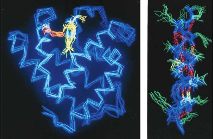
Molecular dynamics simulations (e.g., Fig. 9-32) have re-

vealed that a protein’s native structure really consists of a

large collection of conformational substates that have essen-

tially equal stabilities. These substates, which each have

slightly different atomic arrangements, randomly intercon-

vert at rates that increase with temperature. Consequently,

the interior of a protein typically has a fluidlike character

for structural displacements of up to ⬃2 Å, that is, over ex-

cursions that are somewhat larger than a bond length.

Gregory Petsko and Dagmar Ringe have demonstrated

the functional significance of the internal motions in proteins.

Both experimental and theoretical evidence indicates that

below ⬃220 K (⫺53°C),collective motions in proteins are ar-

rested, leaving atomic fluctuations as the dominant intramol-

ecular motions. For example, X-ray studies have shown that,

at 228 K, the enzyme RNase A, in its crystalline form, readily

binds an unreactive substrate analog (protein crystals gener-

ally contain large solvent-filled channels through which small

molecules rapidly diffuse; at low temperatures, the water is

prevented from freezing by the addition of an antifreeze such

as methanol).Yet, when the same experiment is performed at

212 K,the substrate analog does not bind to the enzyme, even

after 6 days of exposure. Likewise, at 228 K, substrate-free

solvent washes bound substrate analog out of the crystal

within minutes but,if the temperature is first lowered to 212 K,

the substrate analog remains bound to the crystalline enzyme

for at least 2 days. Evidently, RNase A assumes a glasslike

state below 220 K that is too rigid to bind or release substrate.

In terms of landscape theory, this is interpreted as the protein

being trapped in a single energy well.

b. Protein Core Mobility Is Revealed by Aromatic

Ring Flipping

The rate at which an internal Phe or Tyr ring in a protein

undergoes 180° “flips” about its C

␤

¬C

␥

bonds is indicative

of the surrounding protein’s rigidity. This is because, in the

close packed interior of a protein, these bulky asymmetric

groups can move only when the surrounding groups move

aside transiently (although note that these rings have the

shape of flattened ellipsoids rather than thin disks).

NMR spectroscopy can determine the mobilities of pro-

tein groups over a wide range of time scales. Consequently,

the rate at which a particular aromatic ring in a protein flips

is best inferred from an analysis of its NMR spectrum (in-

frequent motions such as ring flipping are not detected by

X-ray crystallography since this technique only reveals the

average structure of a protein). NMR measurements indi-

cate that the ring flipping rate varies from over 10

⫺1

one of immobility (⬍1 s

⫺1

) depending on both the protein

and the location of the aromatic ring within the protein. For

example, bovine pancreatic trypsin inhibitor (BPTI) is a 58-

residue monomeric protein that has eight Phe and Tyr

residues. At 4°C, four of these Phe and Tyr rings flip at rates

⬎5 ⫻ 10

⫺1

, whereas the remaining four rings flip at rates

308 Chapter 9. Protein Folding, Dynamics, and Structural Evolution

Figure 9-32 The internal

motions of myoglobin as

determined by a molecular

dynamics simulation. Several

“snapshots” of the molecule

calculated at intervals of

5 ⫻ 10

⫺12

s are superimposed.

(a) The C

␣

backbone and the

heme group. The backbone is

shown in blue, the heme in

yellow, and the His residue

liganding the Fe in orange.

(b) An ␣ helix.The backbone

is shown in blue, the side

chains in green, and the helix

hydrogen bonds as dashed

orange lines. Note that the

helices tend to move in a

coherent fashion so as to

retain their shape. [Courtesy

of Martin Karplus, Harvard

University.]

(a)

(b)

JWCL281_c09_278-322.qxd 2/24/10 1:17 PM Page 308

ranging between 30 and ⬍1s

⫺1

. These ring-flipping rates

sharply increase with temperature, as expected.

c. Infrequent Motions Can Be Detected through

Hydrogen Exchange

Conformational changes occurring over time spans of

more than several seconds can be chemically characterized

through hydrogen exchange studies (Sections 9-1Cc).

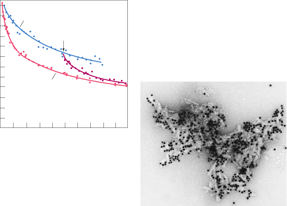
These show that the exchangeable protons of native pro-

teins exchange at rates that vary from milliseconds to many

years (Fig. 9-33). Protein interiors, as we have seen (Section

8-3B), are largely excluded from contact with their sur-

rounding aqueous solvent, and, moreover, protons cannot

exchange with solvent while they are engaged in hydrogen

bonding. The observation that the internal protons of pro-

teins do, in fact, exchange with solvent must therefore be a

consequence of transient local unfolding or “breathing”

that physically and chemically exposes these exchangeable

protons to the solvent. Hence, the rate at which a particular

proton undergoes hydrogen exchange is a reflection of the

conformational mobility of its surroundings. This hypothesis

is corroborated by the observation that the hydrogen ex-

change rates of proteins decrease as their denaturation

temperatures increase and that these exchange rates are

sensitive to the proteins’ conformational states (Fig. 9-33).

5 CONFORMATIONAL DISEASES:

AMYLOID AND PRIONS

Most proteins in the body maintain their native conforma-

tions or,if they become partially denatured, are either rena-

tured through the auspices of molecular chaperones (Sec-

tion 9-2C) or are proteolytically degraded (Section 32-6).

However, ⬃35 different, often fatal, human diseases are as-

sociated with the extracellular deposition of normally solu-

ble proteins in certain tissues in the form of insoluble aggre-

gates known as amyloid (starchlike; a misnomer because it

was originally thought that this material resembled starch).

These include Alzheimer’s disease and Parkinson’s disease,

neurodegenerative diseases that mainly strike the elderly;

the transmissible spongiform encephalopathies (TSEs), a

family of infectious neurodegenerative diseases that are

propagated in a most unusual way; and the amyloidoses, a

series of diseases caused by the deposition of an often mu-

tant protein in organs such as the heart, liver, or kidney.The

deposition of amyloid interferes with normal cellular func-

tion, resulting in cell death and eventual organ failure.

Although the various types of amyloidogenic proteins

are unrelated and their native structures have widely dif-

ferent folds, their amyloid forms have remarkably similar

core structures: Each consists of an array of ⬃10-nm-diam-

eter amyloid fibrils (Fig. 9-34) in which, as infrared, NMR,

and X-ray diffraction methods indicate, certain segments

Section 9-5. Conformational Diseases: Amyloid and Prions 309

123450

Time (h)

Exchangeable H

/heme Fe

Deoxyhemoglobin

Oxyhemoglobin

Figure 9-33 The hydrogen–tritium “exchange-out” curve for

hemoglobin that has been pre-equilibrated with tritiated water.

The vertical axis expresses the ratio of exchangeable protons to

heme Fe atoms. Exchange-out was initiated by replacing the

protein’s tritiated water solvent with untritiated water through

rapid gel filtration (Section 6-3B).As the exchange-out

proceeded, additional gel filtration separations were performed

and the amount of tritium remaining bound to the protein was

measured.At the arrow, O

was added to exchanging

deoxyhemoglobin (hemoglobin lacking bound O

).The changing

slopes of these curves indicate that the hydrogen exchange rates

of the ⬃80 exchangeable protons of each hemoglobin subunit

vary by factors of many decades and that O

binding increases

the exchange rates for ⬃10 of these protons (the structural

changes that O

binding induces in hemoglobin are discussed in

Section 10-2). [After Englander, S.W. and Mauel, C., J. Biol.

Chem. 247, 2389 (1972).]

Figure 9-34 An electron micrograph of amyloid fibrils of the

protein PrP 27–30 (Section 9-5Ce). They are visually

indistinguishable from amyloid fibrils formed by other proteins.

The black dots are colloidal gold beads that are coupled to

anti-PrP antibodies that are adhering to the PrP 27–30. [Courtesy

of Stanley Prusiner, University of California at San Francisco

Medical Center.]

JWCL281_c09_278-322.qxd 2/24/10 1:18 PM Page 309

of the proteins form extended ␤ sheets whose planes ex-

tend parallel to the fibril axis so that their ␤ strands are

perpendicular to the fibril axis (see below).Thus, these pro-

teins each have two radically different stable conformations,

their native forms and their amyloid forms.

We begin this section with a discussion of the amyloi-

doses as exemplified by islet amyloid polypeptide (IAPP;

also called amylin) and certain mutants forms of lysozyme.

We then consider Alzheimer’s disease and finally the TSEs

and their bizarre mode of propagation.

A. Amyloid Diseases

Many amyloidogenic proteins are mutant forms of nor-

mally occurring proteins. These include lysozyme (an en-

zyme that hydrolyzes bacterial cell walls; Section 15-2) in

the disease lysozyme amyloidosis, transthyretin [Fig. 8-66; a

blood plasma protein that functions as a carrier for the

water-insoluble thyroid hormone thyroxin (Section 19-1D)

as well as retinol through its association with retinol bind-

ing protein (Section 8-3Bg)] in familial amyloidotic

polyneuropathy, and fibrinogen (the precursor of fibrin,

which forms blood clots; Section 35-1A) in fibrinogen amy-

loidosis. Most such diseases do not present (become symp-

tomatic) until the third to seventh decades of life and typi-

cally progress over 5 to 15 years ending in death.

a. IAPP Forms a Cross-␤ Spine Structure

IAPP is a 37-residue peptide that is associated with type

2 diabetes mellitus (also called non-insulin dependent and

maturity-onset diabetes mellitus; Section 27-4B), an often

fatal disease that afflicts ⬃100 million mainly older people

worldwide. IAPP is expressed and secreted by the pancre-

atic ␤ islet cells, which also synthesize the polypeptide hor-

mone insulin (Fig. 7-2; whose lack is responsible for type I

or juvenile-onset diabetes mellitis). Although the role of

IAPP in the development of type 2 diabetes is unclear, the

pancreases of 95% of individuals with type 2 diabetes con-

tain amyloid deposits of IAPP with the extent of this depo-

sition increasing with the severity of the disease. Interest-

ingly, mouse IAPP, which differs from human IAPP in 6 of

its 37 residues, does not form amyloid and mice do not de-

velop type 2 diabetes, although transgenic mice that ex-

press human IAPP sometimes do so.

Attempts to crystallize IAPP, either in its native confor-

mation or its amyloid form, have been unsuccesful.

However, through the use of structure prediction tech-

niques (Section 9-3B), Baker and David Eisenberg identi-

fied two of its segments that have high fibril-forming po-

tential: NNFGAIL and SSTNVG, which comprise IAPP’s

residues 21 to 27 and 28 to 33 (5 of the 6 residue differences

between human and mouse IAPP occur in the segment

23–29). Both of these peptides form amyloidlike fibrils as

well as very thin needle-shaped crystals.

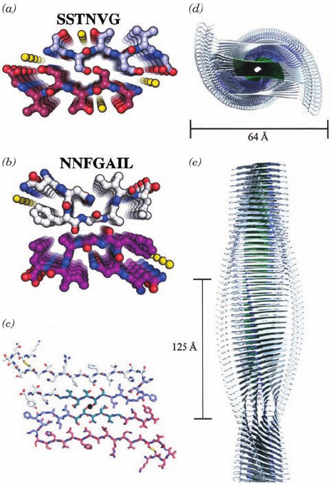
The X-ray structure of SSTNVG, determined by Eisen-

berg, reveals that this hexapeptide forms an extended par-

allel ␤ sheet with two such sheets facing each other such

that their protruding side chains interdigtate so tightly that

they completely exclude water (Fig. 9-35a). The X-ray

structure of NNFGAIL is similar but contains a pro-

nounced bend in its backbone, such that the interface be-

tween the two ␤ sheets is formed between main chains (Fig.

9-35b). Such structures, which are known as cross-␤ spines,

are assumed by a variety of other amyloid-forming pep-

tides, although many of them contain antiparallel rather

than parallel ␤ sheets.

Figures 9-35c–e exhibit a model of the IAPP amyloid

fibril based on the forgoing X-ray structures. Its is a 4-sheet,

310 Chapter 9. Protein Folding, Dynamics, and Structural Evolution

Figure 9-35 The IAPP amyloid fibril. (a) The X-ray structure

of SSTNVG drawn in ball-and-stick form as viewed along the

planes of the ␤ sheets that they form.Atoms are colored

according to type with C on one chain white and the other

magenta, N blue, O red, and water molecules represented by

yellow spheres. (b) The X-ray structure of NNFGAIL viewed

and colored as in Part a.(c) Model of the fibril as viewed along

its axis (black dot).Atoms are colored according to type with the

C atoms of the SSTNVG segment green, those of the NNFGAIL

segment light blue, those of the N-terminal 20 residues and the

C-terminal 4 residues light red or white, N blue, O red, and S

atoms, which form disulfide bonds, yellow. (d) Schematic view

along the fibril axis in which the SSTNVG segments are green,

the NNFGAIL segments are light blue, and the modeled

residues are white. (e) View perpendicular to the fibril axis

represented as in Part d.The helix has a gentle left-handed twist

of 3.4 Å per layer so that it makes a quarter turn every 125 Å.

[Courtesy of David Eisenberg, UCLA. PDBids 3DG1 for

SSTNVG and 3DGJ for NNFGAIL.]

JWCL281_c09_278-322.qxd 2/24/10 1:18 PM Page 310