Vocking B., Alt H., Dietzfelbinger M., Reischuk R., Scheideler C., Vollmer H., Wagner D. Algorithms Unplugged

Подождите немного. Документ загружается.

290 Dominik Sibbing and Leif Kobbelt

The value for the ﬁrst green dot can easily been found:



1,R−



=1+R

− R +

− R

− R.

If we decided to go from a blue point (x, y) in the east direction, the value

of F, evaluated at the green point (x

)=(x +1,y−

), will change in the

following way:

F (x

+1,y

)=(x

+1)

+ y

− R

= x

+2x

+1+y

− R

= F (x

)+2x

+1.

Going in southeast direction, we have to add 1 to the x-coordinate and sub-

tract 1 from the y-coordinate of the green point, so the value of F changes as

follows:

F (x

+1,y

− 1) = (x

+1)

+(y

− 1)

− R

= F (x

)+2x

− 2y

+2.

After these steps we activate the pixel and start the process for the next pixel.

As described, we do not recompute F in very step, but we just update it by

adding small values, depending on the direction we went in. This is called

an “incremental” computation of F , which can be done much faster than

recomputing the whole expression.

Having this in mind we can write down a ﬁrst version of Bresenham’s

Algorithm for circles.

Bresenham’s Algorithm for circles

1(x, y)=(0,R)

2 F =

− R

3 plot(0,R); plot( R, 0)

4 plot(0, −R); plot(−R, 0)

5 while (x<y) do

6 if (F<0) then

7 F = F +2·(x +1)+1

8 x = x +1

9 else

10 F = F +2·(x +1)− 2 · (y −

)+2

11 x = x +1

12 y = y − 1

13 endif

14 plot( x, y); plot( y, x)

15 plot(−x, y); plot( y, −x)

16 plot( x, −y); plot(−y, x)

17 plot(−x, −y); plot(−y,−x)

18 endwhile

29 High-Speed Circles 291

But we can do faster. For both increments (2x

+1) and (2x

− 2y

+2)

we need multiplications. Our algorithm would be faster if we could limit all

calculations to simple additions.

To achieve this we need two more variables, which we call d

and d

so we can track the change of the increments. The idea is that we increase

the function F by d

if we go in the east direction, and by d

if we go in

the southeast direction, which would only require one summation. In addition

to this we also need to change d

and d

depending on the direction we

went in. For both variables we need the initial values, which can be found by

plugging in the initial values of x

and y



1,R−



=2·1+1=3,



1,R−



=2·1 − 2 · R +1+3=5−2 · R.

Nowwehavetothinkabouthowd

and d

will change if we decide

upon one direction. This can be done in a way very similar to changing the

function F itself. Assuming we go in the east direction, both values change in

the following way:

+1,y

)=2·(x

+1)+1=d

)+2,

+1,y

)=2·(x

+1)− 2 · y

+2=d

)+2.

Going in the southeast direction will aﬀect the values for d

and d

follows:

+1,y

− 1) = 2 · (x

+1)+1=d

)+2,

+1,y

− 1) = 2 · (x

+1)− 2 · (y

− 1) + 2 = d

)+4.

The fraction is gratuitous. All the increments are whole numbers, but since the

initial value for F contains a fraction, we carry around this fraction during the

entire process. Since whole numbers can be represented with more accuracy,

it would be nice to just deal with integers.

To ﬁgure out if we can omit the fraction in some way, we consider what

F<0 means. Starting with

F =

− R

and assuming K to be a whole number, we see that F equals K +1/4inevery

step of the computation, since F is only increased by a whole number. So, in

every step F is one of these numbers

F ∈



···, −

, ···



This means, if F drops below zero, then also F − 1/4 drops below zero. So,

instead of starting with F =5/4 − R, we are also allowed to start with

F =1−R, without aﬀecting the correctness of the algorithm.

292 Dominik Sibbing and Leif Kobbelt

The ﬁnal version of Bresenham’s Algorithm for drawing circles uses only

simple summations over whole numbers:

Improved Bresenham’s Algorithm for drawing circles

1(x, y)=(0,R)

2 F =1− R

3 d

4 d

=5− 2 · R

5 plot(0,R); plot( R, 0)

6 plot(0, −R); plot(−R, 0)

7 while (x<y) do

8 if (F<0) then

9 F = F + d

10 x = x +1

11 d

= d

12 d

= d

13 else

14 F = F + d

15 x = x +1

16 y = y − 1

17 d

= d

18 d

= d

19 endif

20 plot( x, y); plot( y, x)

21 plot(−x, y); plot( y, −x)

22 plot( x, −y); plot(−y, x)

23 plot(−x, −y); plot(−y,−x)

24 endwhile

ARacingDuel

Drawing circles with this algorithm works very well: By letting all presented

algorithms compete against each other, one can ﬁgure out that the last algo-

rithm is able to draw circles 14 times faster than the one that was presented

ﬁrst! In addition to that, it just needs summations on whole numbers, which

is useful if we deal with specialized processors. You should try it at home!

There are similar algorithms for other geometric primitives, such as lines

and triangles. These algorithms are integrated as an essential part of current

graphics cards, so displaying detailed pictures at high frame rates becomes

possible for applications such as computer games.

The presented process of ﬁnding an algorithmic solution for a problem

is typical in computer science. First of all it is necessary to ﬁnd a precise

mathematical description of the problem. This makes the implementation of

a simple algorithm for the speciﬁc task possible; it might still have some

29 High-Speed Circles 293

problems (such as gaps in the circle), but it helps us understand the problem

better. After that one can try to ﬁnd a solution, which can be calculated much

faster. Therefore, we can take additional knowledge into account (symmetry

of a circle) or reformulate some equations to simplify some calculations (in-

cremental computation). In the end we can consider architectural properties

of our computer to further accelerate the computations (e.g., summations can

be calculated faster than multiplications). This process might not only lead

to the optimal solution of our speciﬁc problem, it might also give solutions

for similar problems. With some minor changes, the high speed algorithm for

drawing circles can also be used to draw ellipses, parabolas, hyperbolas, or

similar curves used in computer graphics.

Further Reading

1. Chapter 8 (Pledge’s Algorithm) and Chap. 36 (The Smallest Enclosing

Circle)

Results of the presented methods can be illustrated in a graphical sense.

This requires fast rendering algorithms like Bresenham’s Algorithm for

lines and circles, which are capable of drawing geometric primitives.

2. Chapter 11 (Multiplication of Long Integers)

Bresenham’s algorithm for drawing circles does not need any multiplica-

tions. If, however, multiplications become necessary, it should be possible

to calculate them in a fast way. How this works is described in this chapter.

3. Alan Watt: 3D Computer Graphics. Addison-Wesley, 3rd edition, 1999

The book describes basic algorithms from the ﬁeld of computer graphics.

It contains many examples.

4. Mason Woo, Jackie Neider, Tom Davis, Dave Shreiner: The OpenGL Pro-

gramming Guide. Addison-Wesley Professional, 5th edition, 2005.

The book explains techniques far beyond the drawing of simple primitives

and gives an introduction to OpenGL programming. Since it comes with

many examples it motivates the reader to try out diﬀerent techniques.

Gauß–Seidel Iterative Method

for the Computation of Physical Problems

Christoph Freundl and Ulrich R¨ude

Friedrich-Alexander-Universit¨at Erlangen-N¨urnberg, Erlangen, Germany

Warmup: Soccer

The following algorithm deals with the simulation of physical eﬀects. Com-

puters can also be utilized to simulate processes in physics, chemistry, and

anywhere in nature. This is becoming more and more important because it

helps to understand how nature works. For example, our weather forecast

is based on a simulation that attempts to represent the natural weather as

accurately as possible on a computer. New car models and planes are also

simulated, long before they are built for the ﬁrst time. Many scientists actu-

ally completely depend on simulations. Astronomers who want to understand

what happens if two black holes collide have to use computer simulations,

since experiments with real black holes are impossible. Computer games are

also often similar to simulations, only for games it is not necessarily a goal

that the computations coincide with the real world.

Here, we are going to simulate an important problem with our algo-

rithm, namely that of heat distribution, as it would also be important for

weather forecasts. However, we will restrict ourselves to solid bodies like a

two-dimensional plate because it makes the simulation easier to explain if we

do not have to take the air ﬂow into account. But let us ﬁrst start with a

“warmup exercise” and have a look at soccer games.

After having barely missed the ﬁnal round of the last World Cup, the

national team ﬁnally reaches the ﬁnal game four years later. The players are

very nervous, so nervous that the coach is convinced that they will not even

be able to form a line, arranged by shirt numbers, for the national anthem.

As the coach is not allowed to enter the ﬁeld where he could easily put

every player into his place in the line, he desperately comes up with the

following method: he impresses upon the two players with the numbers 1 and

11, which are the left- and rightmost players in the line, to take care that there

is enough space between them for all other players. After that, they shall not

leave their places anymore.

B. V¨ocking et al. (eds.), Algorithms Unplugged,

DOI 10.1007/978-3-642-15328-0

30,

 Springer-Verlag Berlin Heidelberg 2011

296 Christoph Freundl and Ulrich R¨ude

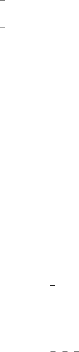
Fig. 30.1. Situation during the line-up: player 5 is being called by the coach. He

moves to the exact middle between his neighbors, the players 4 and 6. The red

dashed line is given by the two players at the boundaries, in the end all players

should stand on it ideally

The other players with the numbers from 2 to 10 receive the following in-

struction: if they are called they shall move to the exact middle between their

right and left neighbors (see Fig. 30.1). The coach calls all players consecu-

tively in the order of their shirt numbers. After the player with the highest

number has moved, the coach starts again from the beginning.

You can try this out yourself quickly, for example with game pawns. The

website for this algorithm contains a program that visualizes this approach.

You will see: after several cycles of this method the players have indeed moved

30 Gauß–Seidel Iterative Method 297

such that they form at least an approximate line. It is not completely perfect

but good enough such that nobody notices it.

In order to get the players exactly onto the line, the algorithm would

have to run for an inﬁnitely long time. This is why you will never get the

completely right result in practice. But that does not matter because after

suﬃciently many steps the algorithm’s outcome can get arbitrarily close to

the correct solution. You encounter algorithms like this often when it comes

to so-called numerical problems, i.e., when real decimal numbers have to be

computed, such as those needed by physicists or engineers.

If the players line up in the order of their back numbers, they will be

called from left to right over and over again but we can also do it diﬀerently.

A popular variant is the so-called red-black ordering of the players. There the

half of the players with the lower numbers occupy every other place in the

line ﬁrst, then the players with the high numbers ﬁll up the remaining places.

But even if the players are arranged completely at random, the method still

works, only it must be obvious to every player who both his neighbors are.

This method is the algorithm of Gauß and Seidel, which we are going to

apply for physical problems in the following.

Temperature Calculation in a Rod (1D)

Now, let us really consider the calculation of a temperature distribution. Is it

not somewhat amazing that we can use the principle of lining up in a row?

For example, if you look at the temperature distribution in a thin rod you will

notice that the temperature at every point along the rod is the average of the

temperatures in the neighborhood of that point. If you ﬁx the temperature

at both ends of the rod, the temperature between both ends runs “in a row”,

i.e., linearly from one end to the other.

In order to compute this linear distribution of values, you need not use a

computer, just as a soccer coach needed no complicated algorithm in order

to place players in a row. But we can now see that the problems are related,

and maybe they can be solved in the same way. Observe that the position of

a player corresponds to a temperature value, otherwise the computation can

proceed in the same way as in our soccer problem.

Next, we make the task a bit more interesting: how does the temperature

distribution look if we heat the rod at some point in the middle? Then the

temperature at that point is of course no longer the average of the neighboring

temperatures, the additional heating has to be taken into account.

Now there is no longer an obvious possibility to determine the resulting

temperature distribution so we ponder how to utilize the computer for solving

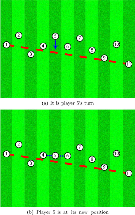
this problem. A ﬁrst diﬃculty is posed by the fact that there are inﬁnitely

many points along the rod, however a computer can only treat ﬁnitely many

objects in ﬁnite time. Therefore, we choose a ﬁnite number of points along

the rod (see Fig. 30.2) at which we want to compute the temperature. This

298 Christoph Freundl and Ulrich R¨ude

Fig. 30.2. Discretization of a continuous rod with 11 points

method is also called discretization as we are mapping a continuous problem

to a discrete problem.

If the points are distributed evenly along the rod, and if u

denotes the

temperature value and f

the heating at point i, then the temperature at a

particular point is updated by the formula

i−1

+ u

i+1

)+f

The algorithm GaussSeidel1D

1 procedure GaussSeidel1D (n, u, f)

2 begin

3 for i := 2 to n − 1 do

4 u[i]:=

(u[i − 1] + u[i +1])+f [i]

5 endfor

6 end

Like in the example of the soccer players only the points in the interior

of the rod are continuously recalculated, we assume the temperatures at both

boundary points of the rod are given. Depending on the physical experiment

it could also be the case that the temperatures at the rod’s boundaries are

30 Gauß–Seidel Iterative Method 299

not ﬁxed. We also have not considered that in practice the rod would lose

some heat to its neighborhood. We could take that into account by using

correspondingly more complicated formulas and computations, but that would

lead us too far for now. Instead, we will investigate another diﬃculty which

arrives if we do not want to compute the temperature distribution in a one-

dimensional rod, but in a two-dimensional plate.

Temperature Computation on a Plate (2D)

We can generalize the formulation of the task by leaving the one-dimensional

rod behind and will now consider a two-dimensional cooking plate, which

might again be heated at some places.

The discretization works similarly to the above case, only now we get a

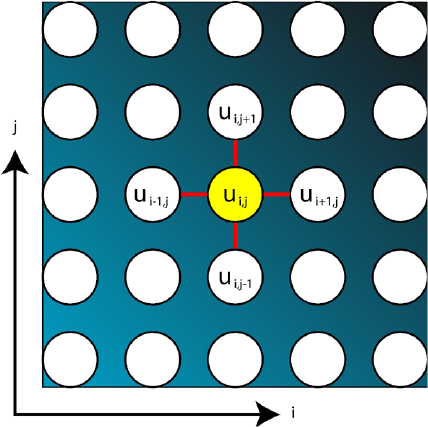
two-dimensional grid of points. We want to compute the temperature at these

points. Averaging the neighboring temperatures at particular points means

now to take not only the right and left neighbors into account but also the

upper and lower neighbors (see Fig. 30.3).

Because of this representation of the dependencies of a point with respect

to its neighboring points one identiﬁes the stencil which has to be applied to

the point and its surrounding in order to recompute its value. In this case we

have a ﬁve-point stencil (because it involves ﬁve neighboring points), and the

Fig. 30.3. Schematic view of a discretized two-dimensional plate and the ﬁve-point

stencil