Vocking B., Alt H., Dietzfelbinger M., Reischuk R., Scheideler C., Vollmer H., Wagner D. Algorithms Unplugged

Подождите немного. Документ загружается.

310 Norbert Blum and Matthias Kretschmer

to y[0]. Since the algorithm will choose the third possible mutation in the last

step, it will generate the solution which we have intuitively generated.

The lines in the table that form a path from cell (0, 0) to a cell (i, j),

represent the possible transformations from x[i]toy[j]. In the case of (2, 1),

we used the path over (1, 0) by ﬁrst deleting A and then substituting T by T.

The table shows that there might be multiple paths to a cell (i, j). Hence, there

might exist multiple diﬀerent optimal sequences of mutations to transform x

to y. The lines can be calculated by the algorithm, as these just represent

the case that lead to a minimum distance in a single step. The red colored

lines constitute the path of minimum cost for the transformation of x to y.

Hence, these represent the sequences of mutations that transform x to y with

minimum cost and which can be used to get the evolutionary distance.

We do not know which cells we require for the calculation of a path of

minimum cost to transform x to y. Thus, we have to calculate the values of

all cells. To calculate the value d

(x[i],y[j]) of cell (i, j), we need the values

of the cells (i − 1,j), (i, j − 1) and (i − 1,j − 1). To make sure that we have

already calculated these values, we generate the table row by row or column

by column. If we do it row by row, we need to go through the rows from

the left to the right. Similarly, if we generate the table column by column,

we need to go through the columns from the top to the bottom. This ensures

that all required values are stored in the table, when we calculate the distance

(x[i],y[j]). At the end, the evolutionary distance d

(x[m],y[n]) = d

(x, y)is

stored in the cell (m, n).

Conclusion

Starting with the smallest subproblem, the calculation of d

(x[0],y[0]), we

have solved larger and larger subproblems. In each step we have increased the

lengths of the preﬁxes of x and y and calculated their evolutionary distances.

For the calculation of the distance d

(x[i],y[j]) we have used the distances

(x[i − 1],y[j]), d

(x[i],y[j − 1]) and d

(x[i − 1],y[j − 1]). Hence, we have

used the optimal solution of these smaller subproblems to solve the larger

subproblem.

Given a problem, the calculation of a solution of minimum cost is called an

optimization problem. The calculation of the evolutionary distance of two DNA

sequences is such an optimization problem. We have used a speciﬁc technique

to create an algorithm for our optimization problem. This generic technique

may be applied to other but not all optimization problems. Implicitly, we have

used the following property of our optimization problem:

• Every subsolution of an optimal solution which is a solution for a subprob-

lem is an optimal solution for that subproblem.

Many optimization problems have this property. The technique we have used

for solving the problem of ﬁnding the evolutionary distance may be applied

31 Dynamic Programming – Evolutionary Distance 311

to any problem with this property. This technique is called dynamic pro-

gramming. In the case of dynamic programming, we split the problem into

subproblems. We solve the smallest subproblems directly. In our case, this is

the calculation of d

(x[0],y[0]). The solution for this subproblem is zero. From

the optimal solutions of small subproblems we calculate the optimal solutions

of larger subproblems. We repeat this until we have calculated the optimal so-

lution of the original problem. Dynamic programming is an important generic

technique that is often used for the development of algorithms.

The algorithm for calculating the minimum evolutionary distance of two

DNA sequences can be used for other purposes than calculating the similarity

of two species. For example, one can use it to measure the similarity of two

words. This can be useful for spellchecking software. The correct spelling of a

word has most probably a very small distance to the incorrectly spelled word

given by the user. So the software may show the user all words within a given

maximum distance as possible correct spellings of the given word.

References

The references below provide a generic introduction to dynamic programming.

They present the theoretical background and also examples of its application.

1. Thomas H. Cormen, Charles E. Leiserson, Ronald L. Rivest and Cliﬀord

Stein: Introduction to Algorithms. MIT Press, 2nd edition, 2001. Chap-

ter 3.

2. Jon Kleinberg,

Eva Tardos: Algorithm Design. Addison-Wesley, 2005.

Chapter 6.

Part IV

Optimization

Overview

Heribert Vollmer and Dorothea Wagner

Universit¨at Hannover, Hannover, Germany

Karlsruher Institut f¨ur Technologie, Karlsruhe, Germany

How can we ﬁnd the shortest way to go from one city to another? How can

we ﬁnd the order in which to visit diﬀerent cities such that the resulting

round tour is the shortest among all possibilities? In the ﬁnal part of this

book we look at such tasks where, given a generally very large set of “possible

solutions” to an algorithmic goal, we have to determine in a certain sense

the “optimal solution.” In computer science, such problems are known as

optimization problems.

We will see that for many optimization problems very tricky algorithms

are known that produce an optimal solution very quickly (“eﬃciently”). The

above-mentioned shortest-path problem is one of them. In Chap. 32 an algo-

rithm for this and related problems will be presented. Also the subsequent six

chapters of the ﬁnal part of this book explain eﬃcient procedures to ﬁnd so-

lutions for diﬀerent optimization problems. In Chap. 33 some islands have to

be connected via a system of bridges in such a way that it is possible to drive

from each island to each other, but the number and size of the bridges has to

be as small as possible. Chapter 34 explains how car traﬃc can be distributed

among the diﬀerent streets of a city with diﬀerent numbers of lanes in such

a way that we have as few traﬃc jams as possible. This is an example of a

so-called network ﬂow problem – these problems are of immense importance

in computer science today. The task of a dating service to arrange meetings

among marriage-minded ladies and gentlemen is solved optimally (at least

from a theoretical point of view) in Chap. 35. In Chap. 36 we must choose

the location for a new suburban ﬁre brigade headquarters.

Finally we have to ﬁnd solutions for optimization problems where the

problem speciﬁcation is not completely known from the beginning. For these

online problems the parameters become known only little by little. In Chap. 37

we have to decide if, for a skiing holiday, it is better to buy or rent the skis,

but we do not know yet if we will reuse the skis later. In Chap. 38 we want to

move, and we want to use as few boxes as possible to pack our stuﬀ, but we

are not fully decided yet which things we want to move and which we want

to throw away.

B. V¨ocking et al. (eds.), Algorithms Unplugged,

DOI 10.1007/978-3-642-15328-0,

 Springer-Verlag Berlin Heidelberg 2011

316 Heribert Vollmer and Dorothea Wagner

For many other important optimization problems no eﬃcient solution al-

gorithm is known to this day. The only way to ﬁnd the optimal solution is to

compare all possible solutions. The time requirement for this simple proce-

dure is of course dependent on the number of solutions and hence in general

it is very large. For example, in Chap. 39 a knapsack has to be packed opti-

mally for a hike, but there are many diﬀerent ways to use its capacity. Also

the above problem to determine the shortest round-trip through a number

of cities is one of the hard problems for which we do not know how to ﬁnd

an optimal solution. But in Chap. 40 we will see how a so-called approxi-

mation algorithm ﬁnds a tour that is maybe not the shortest one but one

whose length usually is quite close to the optimum; in the worst case it is

twice as long. The ﬁnal chapter of this book, Chap. 41, introduces simulated

annealing, an algorithmic method that produces approximate solutions for a

number of optimization problems with certain mathematical properties. The

name of this magical method is due to an analogy with an industrial technique

that involves the heating and controlled cooling (“annealing”) of a material

to improve its stability.

Shortest Paths

Peter Sanders and Johannes Singler

Karlsruher Institut f¨ur Technologie, Karlsruhe, Germany

I have just moved to Karlsruhe and into my ﬁrst ﬂat. Such a big city is rather

complicated. I already have a city map, but how can I ﬁnd the fastest way

to get from A to B? I like cycling but I am notoriously impatient, so I really

need the shortest path to the university, to my girlfriend, and so on.

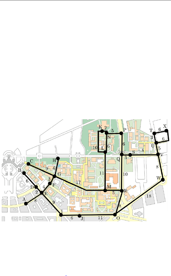
Systematic planning could look like this: I pin the city map on a table

and put thin yarn threads along the streets, knotting them at crossroads and

junctions. I also knot all possible start points, end points and dead ends.

Fernerkundung

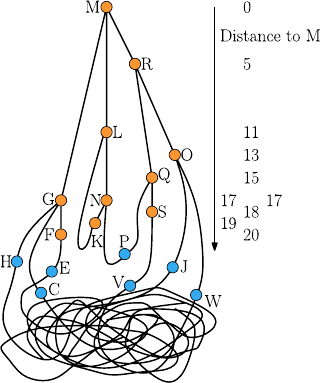
Here comes the trick: I pick the starting knot and slowly lift it up. One

after another the knots leave the table surface. I have labeled the nodes so that

B. V¨ocking et al. (eds.), Algorithms Unplugged,

DOI 10.1007/978-3-642-15328-0

32,

 Springer-Verlag Berlin Heidelberg 2011

318 Peter Sanders and Johannes Singler

I always know where each knot comes from. At last, all knots hang vertically

below the starting knot.

The rest is really easy: To ﬁnd the shortest path, I only have to ﬁnd the end

knot and trace the straight threads back to the start. The distance between

both points can then be found with a measuring tape. The path found this

way must indeed be the shortest, because if there was a shorter one, it would

have kept the start and end closer together.

Suppose, for example, I need the shortest path from the cafeteria (M) to

the computing center (F). I pick knot M, lifting all other knots oﬀ the table.

The ﬁgure below shows the situation at the moment when knot F hangs in

the air for the ﬁrst time. To make the ﬁgure clearer, the knots are pulled

apart horizontally a bit. The orange knots are hanging, the numbers on the

right indicate the distance to M using the thread length from the ﬁrst ﬁg-

ure.

It is obvious that the shortest path from M to F leads via G. Between L

and K, the thread is already sagging with no chance of hanging any straighter.

This means there is no shortest path from M using this connection.

I have tried this method successfully for the campus and its surroundings.

But I failed miserably with my ﬁrst trial run for the whole city of Karlsruhe,

which produced nothing but a heap of tangled threads. It took me half the

night to disentangle them and lay them out on the city map again.

My younger brother drops by the next day. “No problem,” he says, “I will

solve the problem with superior technology!” He turns to his chemical kit and

soaks the threads in a mysterious liquid. Good grief! He ignites the web at

the starting point. Seconds later, the room disappears in a cloud of smoke.

This pyromaniac turned the threads into fuses. He explains proudly: “All

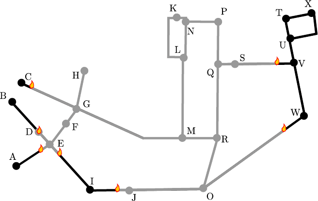
32 Shortest Paths 319

threads are burning at the same speed. So the time before a knot catches ﬁre

is proportional to the distance from the starting point. Besides, the direction

from which a knot catches ﬁre contains the same information as the straight

threads of my hanging web approach.” Great! Unfortunately, he forgot to

record the inferno, so we have only ashes left. Even with a video tape I would

have to start over with every new starting point. Below, there is a snapshot

of the threads after the ﬂames from starting point M have burned part of the

way (gray).

I throw my brother out and start to think. I have to get over my fear of

abstraction and make the problem clear to my stupid computer. This does

have certain advantages: threads that do not exist cannot get tangled up or

burn. My professor told me that back in 1959 a certain Mr. Dijkstra developed

an algorithm that solves the shortest-path problem in a way that is quite

similar to the thread method. Neatly enough, Dijkstra’s algorithm can be

described in thread terminology.

Dijkstra’s Algorithm

Mainly, it is about simulating the thread algorithm. For every knot, a com-

puter implementation must know the threads starting from it and their re-

spective lengths. It also administrates a table d which estimates the distance

from the starting point. The distance d[v] is the length of the shortest connec-