Vidakovic B. Statistics for Bioengineering Sciences: With Matlab and WinBugs Support

Подождите немного. Документ загружается.

16.2 Simple Linear Regression 611

SSE

−2,1−α/2

SSE

−2,α/2

The following part of MATLAB script tests H

: σ

=0.5 versus H

: σ

<0.5

and ﬁnds a 95% conﬁdence interval for

. As is evident, H

is not rejected (p-

value 0.1981), and the interval is [0.2741,0.6583].

%test H

0: sigma2 = 0.5 vs H

1: sigma2 < 0.5

ch2 = SSE/0.5 %33.1981

ptst3 = chi2cdf(ch2, n-p) %0.1981

% Find 95% CI for sigma2

[SSE/chi2inv(0.975, n-p), SSE/chi2inv(0.025, n-p)]

% 0.2741 0.6583

16.2.1.4 Inference About the Mean Regression Response for x = x

∗

Suppose that the regression

y = b

x has been found and that we are inter-

ested in making an inference about the response y

=E(y|x = x

∗

) =β

+β

∗

The statistic for y

= b

∗

, and it is a random variable since both

and b

are random variables.

The

is an unbiased estimator of y

, E

=E(b

∗

) =β

+β

∗

= y

as expected. The variance of

is obtained from representation

= b

∗

= y+b

∗

−x) and the fact that the correlation between y and b

is zero:

Var

=σ

∗

−x)

Thus,

∼N

+β

∗

,σ

∗

−x)

¶¶

from which we develop the inference.

The test

: y

= y

relies on the statistic

− y

∗

−x)

612 16 Regression

This statistic under H

has a t-distribution with n −2 degrees of freedom and

testing is done as in the cases of

and β

The (1 −α)100% conﬁdence interval for y

=β

+β

∗

−t

n−2,1−α/2

∗

−x)

n−2,1−α/2

∗

−x)

16.2.1.5 Inference About a New Response for x

= x

∗

Suppose that the regression

y = b

x has been established and that we

are interested in predicting the response

pred

for a new observation, cor-

responding to a covariate x

= x

∗

. Given the value x = x

∗

, the difference be-

tween the inference about the mean response y

discussed in the previous

section and the inference about an individual outcome y

pred

is substantial.

As in the previous subsection,

pred

= b

+ b

∗

, and the mean of

pred

) =β

+β

∗

= y

pred

, which is in fact equal to y

Where y

pred

and y

differ is their variability. The variability of

pred

has

two sources, ﬁrst, the variance of the distribution of ys for x

= x

∗

, which is

, and second, the variance of sampling distribution for b

∗

, which is

∗

−x)

. Thus, Var (

pred

) = MSE +Var (

The distribution for

pred

is normal,

pred

∼N

+β

∗

,σ

1 +

∗

−x)

¶¶

and the subsequent inference is based on this distribution.

The test

: y

pred

= y

relies on the statistic

pred

− y

1 +

∗

−x)

This statistic under H

has a t-distribution with n −2 degrees of freedom,

which implies the inference.

16.2 Simple Linear Regression 613

The (1 −α)100% conﬁdence interval for y

pred

−t

n−2,1−α/2

1 +

∗

−x)

pred

n−2,1−α/2

1 +

∗

−x)

% predicting y for the new observation x, CI and PI

newx = 230; %Deficit = 230

newx = b0 + b1

newx % 16.5195

sym = s

sqrt(1/n + (mean(x) - newx)^2/SXX )

%st.dev. for mean response, sym = 3.2839

syp = s

sqrt(1 + 1/n + (mean(x) - newx)^2/SXX )

%st.dev. for the prediction syp = 3.3450

alpha = 0.05;

%mean response interval

lbym = y

newx - tinv(1-alpha/2, n-p)

sym;

rbym = y

newx + tinv(1-alpha/2, n-p)

sym;

% prediction interval

lbyp = y

newx - tinv(1-alpha/2, n-p)

syp;

rbyp = y

newx + tinv(1-alpha/2, n-p)

syp;

% the intervals

[lbym rbym] % 9.8875 23.1516

[lbyp rbyp] % 9.7642 23.2749

Next, we will ﬁnd Bayesian estimators of regression parameters in the

same example, Diabetes Mellitus in Children, by using WinBUGS. On p. 606

we mentioned that taking x

−x as a predictor instead of x

is beneﬁcial in the

Bayesian context. From such a parametrization of regression,

=β

∗

+β

−x) +²

the traditional intercept

is easily obtained as β

∗

−β

model{

for (i in 1:ntotal){

y[i] ~ dnorm( mui[i], tau )

mui[i] <- bb.0 + b.1

(x[i] - mean(x[]))

yres[i] <- y[i] - mui[i]

}

bb.0 ~ dnorm(0, 0.0001)

b.0 <- bb.0 - b.1

mean(x[])

b.1 ~ dnorm(0, 0.0001)

tau ~ dgamma(0.001, 0.001)

s <- 1/sqrt(tau)

}

DATA

614 16 Regression

list(ntotal=43,

y = c(4.8, 4.1, 5.2, 5.5, 5.0, 3.4, 3.4, 4.9, 5.6, 3.7,

3.9, 4.5, 4.8, 4.9, 3.0, 4.6, 4.8, 5.5, 4.5, 5.3,

4.7, 6.6, 5.1, 3.9, 5.7, 5.1, 5.2, 3.7, 4.9, 4.8,

4.4, 5.2, 5.1, 4.6, 3.9, 5.1, 5.1, 6.0, 4.9, 4.1,

4.6, 4.9, 5.1),

x = c(-8.1, -16.1, -0.9, -7.8, -29.0, -19.2, -18.9, -10.6,

-2.8, -25.0, -3.1, -7.8, -13.9, -4.5, -11.6, -2.1,

-2.0, -9.0, -11.2, -0.2, -6.1, -1.0, -3.6, -8.2,

-0.5, -2.0, -1.6, -11.9, -0.7, -1.2, -14.3, -0.8,

-16.8, -5.1, -9.5, -17.0, -3.3, -0.7, -3.3, -13.6,

-1.9, -10.0, -13.5))

INITS

list(bb.0 = 0, b.1 = 0, tau=1)

The output is given in the table below. It contains Bayesian estimators b.0

for β

and b.1 for β

. In the least-squares regression we found b

= S

0.0494, b

= y−b

·x =5.1494, and s =

MSE =0.6363. Since priors were non-

informative, we expect that Bayesian estimators will be close to the classical.

Indeed that is the case:

b.0 = 5.149, b.1 = 0.0494, and s = 0.6481.

The classical standard errors of estimators for

and β

are sb0 = 0.1484

and sb1 = 0.0138, while the corresponding Bayesian estimators are 0.1525

and 0.01418.

The classical 95% conﬁdence interval for

was found to be [0.0216,0.0773].

The Bayesian 95% credible set for

is [0.02139,0.07733], as is evident from

val2.5pc and val97.5pc in the output below.

mean sd MC error val2.5pc median val97.5pc start sample

b.0 5.149 0.1525 3.117E-4 4.848 5.149 5.449 2001 200000

b.1 0.0494 0.0141 3.072E-5 0.02139 0.04944 0.07733 2001 200000

s 0.6481 0.0734 1.771E-4 0.5236 0.6415 0.811 2001 200000

yres[1] 0.05111 0.09944 2.175E-4 -0.1444 0.05125 0.2472 2001 200000

yres[2] -0.2537 0.1502 3.459E-4 -0.5499 -0.2533 0.0418 2001 200000

yres[3] 0.09544 0.1431 2.925E-4 -0.1861 0.09505 0.378 2001 200000

yres[4] 0.7363 0.09957 2.167E-4 0.5406 0.7364 0.9325 2001 200000

...

yres[41] -0.4552 0.1333 2.727E-4 -0.7173 -0.4555 -0.1919 2001 200000

yres[42] 0.245 0.1028 2.314E-4 0.04251 0.2451 0.4475 2001 200000

yres[43] 0.6179 0.125 2.879E-4 0.3718 0.6179 0.8632 2001 200000

Thus, the Bayesian approach to regression estimation is quite close to the

classical when the priors on

and β

and the precision τ =1/σ

are noninfor-

mative.

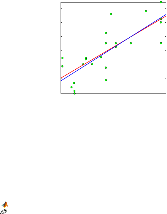
Example 16.2. Hubble Telescope and Hubble Regression. Hubble’s con-

stant (H) is one of the most important numbers in cosmology because it is

instrumental in estimating the size and age of the universe. This long-sought

number indicates the rate at which the universe is expanding, from the pri-

mordial “Big Bang.” The Hubble constant can be used to determine the intrin-

sic brightness and masses of stars in nearby galaxies, examine those same

16.2 Simple Linear Regression 615

properties in more distant galaxies and galaxy clusters, deduce the amount of

dark matter present in the universe, obtain the scale size of faraway galaxy

clusters, and serve as a test for theoretical cosmological models.

Fig. 16.4 Edwin Powell Hubble (1889–1953).

In 1929, Edwin Hubble

(Fig. 16.4) investigated the relationship between

the distance of a galaxy from the Earth and the velocity with which it ap-

pears to be receding. Galaxies appear to be moving away from us no matter

which direction we look. This is thought to be the result of the “Big Bang.”

Hubble hoped to provide some knowledge about how the universe was formed

and what might happen in the future. The data collected included distances

(megaparsecs

) to n =24 galaxies and their recessional velocities (km/sec).

Hubble’s law is as follows: Recessional velocity = H

× distance,

where H is Hubble’s constant (units of H are [km/sec/Mpc]). By working back-

ward in time, the galaxies appear to meet in the same place. Thus 1/H can be

used to estimate the time since the Big Bang – a measure of the age of the

universe.

Distance in megaparsecs ([Mpc]) 0.032 0.034 0.214 0.263 0.275 0.275

0.45 0.5 0.5 0.63 0.8 0.9

0.9 0.9 0.9 1.0 1.1 1.1

1.4 1.7 2.0 2.0 2.0 2.0

Recessional velocity ([km/sec]) 170 290 −130 −70 −185 −220

200 290 270 200 300 −30

650 150 500 920 450 500

500 960 500 850 800 1090

A regression analysis seems appropriate; however, there is no intercept

term in Hubble’s law. Can you verify that the constant term of the regression

analysis is not signiﬁcantly different than 0 at any reasonable

level of α. Find

Edwin Powell Hubble (b. Nov. 20, 1889, Marshﬁeld, Missouri, U.S., d. Sept. 28, 1953, San

Marino, California.), American astronomer who is considered the founder of extragalactic

astronomy and who provided the ﬁrst evidence of the expansion of the universe.

1 parsec = 3.26 light years

Reasonable here means level α not larger than 0.10

616 16 Regression

the 95% conﬁdence interval for the slope β

, also known as Hubble’s constant

H, from the given data.

The age of the universe as predicted by Hubble (in years) is about 2.3 bil-

lion years.

0 0.5 1 1.5 2

−200

200

400

600

800

1000

Velocity (km/s)

Distance (mps)

Fig. 16.5 Hubble’s data and regression ﬁts. The blue line is an unconstrained regression

(with intercept ﬁtted), and the red line is a no-intercept ﬁt. The slope for the no-intercept ﬁt

is b

=423.9373 (=H).

%H = 423.9373

secinyear =60

365 %31536000

kminmps = 3.08568025

10^19;

age = 1/H

kminmps/secinyear %2.3080e+009

Modern measurements put H at approx. 70, thus predicting the age of the

universe to about 14 billion years.

Figure 16.5 showing Hubble’s data and regression ﬁts is generated by

hubble.m.

16.3 Testing the Equality of Two Slopes*

Let (x

, y

), i =1,..., n

and (x

, y

), i =1,..., n

, be the pairs of measure-

ments obtained from two groups, and for each group the regression is esti-

mated as

= b

0(1)

1(1)

i(1)

, i =1,.. . , n

, and

= b

0(2)

1(2)

i(2)

, i =1,.. . , n

16.3 Testing the Equality of Two Slopes* 617

where in groups i = 1,2 the statistics b

0(i)

and b

1(i)

are estimators of the re-

spective population parameters, intercepts

0(i)

, and slopes β

1(i)

. We are inter-

ested in testing the equality of the population slopes,

: β

1(1)

=β

1(2)

against the one- or two-sided alternatives.

The test statistic is

1(1)

−b

1(2)

s.e.(b

1(1)

−b

1(2)

)

, (16.2)

where the standard error of the difference b

1(1)

−b

1(2)

s.e.(b

1(1)

−b

1(2)

) =

xx(1)

xx(2)

and s

is the polled estimator of variance,

SSE

+SSE

−4

Statistic t in (16.2) has a t-distribution with n

−4 degrees of freedom

and, in addition to testing, could be used for a (1

−α) 100% conﬁdence interval

for

1(1)

−β

1(2)

[(b

1(1)

−b

1(2)

) ∓t

−4,1−α/2

×s.e.(b

1(1)

−b

1(2)

)].

Example 16.3. Cadmium Poisoning. Chronic cadmium poisoning is an in-

sidious disease associated with the development of emphysema and the excre-

tion in the urine of a characteristic protein of low molecular weight. The ﬁrst

signs of chronic cadmium poisoning become apparent following a latent in-

terval after exposure has ended. Respiratory functions deteriorate faster with

in age. The data set featured in Armitage and Berry (1994) gives ages (in

years) and vital capacity (in liters) for 84 men working in the cadmium indus-

try,

cadmium.dat|mat|xlsx. The observations with ﬂag exposure equal to 0

denote persons unexposed to cadmium oxide fumes, while ﬂags 1 and 2 corre-

spond to exposed persons. The purpose of the study was to assess the degree

of inﬂuence of exposure to respiratory functions. Since respiratory functions

are inﬂuenced by age, regardless of exposure, age as a covariate needs to be

taken into account. Thus, the suggested methodology is to test the equality of

the slopes in group regressions of vital capacity to age:

: β

1(exposed)

=β

1(unexposed)

versus H

: β

1(exposed)

<β

1(unexposed)

618 16 Regression

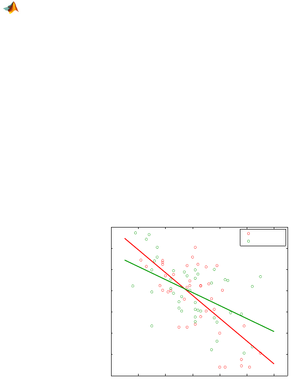
The research hypothesis is that the regression in the exposed group is “steeper,”

that is, the vital capacity decays signiﬁcantly faster with age. This corresponds

to a smaller slope parameter for the exposed group since in this case the slopes

are negative (Fig. 16.6). The inference is supported by the following MATLAB

code.

xlsread vitalcapacity.xlsx;

twos = ans;

x1 = twos( twos(:,3) > 0, 1); y1 = twos( twos(:,3) > 0, 2);

x2 = twos( twos(:,3) ==0, 1); y2 = twos( twos(:,3) ==0, 2);

n1=length(x1); n2 = length(x2);

SXX1 = sum((x1 - mean(x1)).^2) %4.3974e+003

SXX2 = sum((x2 - mean(x2)).^2) %6.1972e+003

SYY1 = sum((y1 - mean(y1)).^2) %26.5812

SYY2 = sum((y2 - mean(y2)).^2) %20.6067

SXY1 = sum((x1 - mean(x1)).

(y1 - mean(y1))) %-236.3850

SXY2 = sum((x2 - mean(x2)).

(y2 - mean(y2))) %-189.7116

1 = SXY1/SXX1 %-0.0538

2 = SXY2/SXX2 %-0.0306

SSE1 = SYY1 - (SXY1)^2/SXX1 %13.8741

SSE2 = SYY2 - (SXY2)^2/SXX2 %14.7991

s2 = (SSE1 + SSE2)/(n1 + n2 - 4) %0.3584

s = sqrt(s2) %0.5987

seb1b2 = s

sqrt( 1/SXX1 + 1/SXX2 ) %0.0118

t = (b1

1 - b1

2)/seb1b2 %-1.9606

pval = tcdf(t, n1 + n2 - 4) %0.0267

10 20 30 40 50 60 70

2.5

3.5

4.5

5.5

age (years)

VC (liters)

exposed

unexposed

Fig. 16.6 Samples from exposed (red) and unexposed (green) groups with ﬁtted regression

lines. The slopes of the two regressions are signiﬁcantly different with a p-value smaller

than 3%.

16.4 Multivariable Regression 619

Thus, the hypothesis of equality of slopes is rejected with a p-value of

2.67%.

Note. Since the distribution of t-statistic is calculated under H

, which

assumes parallel regression lines, the more natural estimator

s22, in place of

s2, takes into account this fact. The number of degrees of freedom in the t-

statistic changes to n

−3. The changes in the inference are minimal, as

evidenced from the MATLAB code accounting for

s22.

%s22 accounts for equality of slopes:

s22 = (SYY1 + SYY2 - ...

(SXY1 + SXY2)^2/(SXX1 + SXX2))/(n1 + n2 - 3) %0.3710

s = sqrt(s22) %0.6091

seb1b2 = s

sqrt( 1/SXX1 + 1/SXX2 ) %0.0120

t = (b1

1 - b1

2)/seb1b2 %-1.9270

pval = tcdf(t, n1 + n2 - 3) %0.0287

For the case of the conﬁdence interval, estimator s2 and n

−4 degrees

of freedom should be used.

16.4 Multivariable Regression

It is often the case that in an experiment leading to regression analysis more

than a single covariate is available. For example, in Chap. 2, p. 31, we dis-

cussed an experiment in which two indices of the amount of body fat (Siri

and Brozek indices) were calculated from the body density measure. In ad-

dition, a variety of body measurements, including weight, height, adiposity,

neck, chest, abdomen, hip, thigh, knee, ankle, biceps, forearm, and wrist, were

recorded. Recall that the body density measure is complicated and potentially

unpleasant, since it is taken by submerging the subject in water. Therefore, it

is of interest to ask whether the Brozek index can be well predicted using the

nonintrusive measurements.

If x

, x

,... , x

are variables, covariates, or predictors, and we have n joint

measurements of covariates and the response, x

, x

,... , x

, y

, i =1,2,..., n,

then multivariable regression expresses the response as a linear combination

of covariates, plus an intercept and an additive error:

=β

+β

+···+β

+²

, i =1,.. . , n.

The errors

are assumed to be independent and normal with mean 0 and

constant variance

. We will denote by k the number of covariates, but the

number of parameters in the model is p

= k+1 because the intercept β

should

be added. To avoid confusion we will mostly use p – the number of parameters

in all expressions that involve dimensions and derived statistics.

As in the univariate case, we will be interested in estimating and test-

ing the coefﬁcients, error variance, and mean and prediction responses. How-

620 16 Regression

ever, multivariable regression brings several new challenges when compared

to a simple regression. The two main challenges are (i) the possible presence

of multicollinearity among the covariates, that is, covariates being correlated

among themselves, and (ii) a multitude of possible models and the need to ﬁnd

the best model by identifying the “best” subset of predictors. A synonym for

multivariable regression is multivariate regression, although the second term

is also used when the response y is multivariate, which is not the case here.

16.4.1 Matrix Notation

If the regression equations for all n observations (x

, x

,... , x

, y

), i =1,.. . , n

are written as

= β

+β

+···+β

+²

= β

+β

+···+β

+²

= β

+β

+···+β

+²

then one can write the above system in convenient matrix form as

= Xβ +²,

where































1 x

··· x

1 x

··· x

1 x

··· x







, β =













, and ² =













Note that y and

² are n×1 vectors, X is an n×p matrix, and β is a p×1 vector.

Here p

= k+1. To ﬁnd the least-squares estimator of β, one minimizes the sum

of squares:

i=1

−(β

+β

+···+β

))