Vidakovic B. Statistics for Bioengineering Sciences: With Matlab and WinBugs Support

Подождите немного. Документ загружается.

530 13 Goodness-of-Fit Tests

Phillips, D. P. (1972). Deathday and birthday: an unexpected connection. In: Tanur, J. M. ed.

Statistics: a guide to the unknown. Holden-Day, San Francisco, 52–65.

Risebrough, R. W. (1972). Effects of environmental pollutants upon animals other than man.

Proc. Sixth Berkeley Symp. on Math. Statist. and Prob., vol. 6, 443–453.

Smirnov, N. (1939). On the estimation of the discrepancy between empirical curves of distri-

bution for two independent samples. Bull. Math. Univ. Moscou, 2, 3–14.

Stansﬁeld, W. D. and Carlton, M. A. (2007). Human sex ratios and sex distribution in sib-

ships of size 2. Hum. Biol., 79, 255–260.

Struhsaker, T. T. (1965). Behavior of the vervet monkey (Cercopithecus aethiops). Ph.D. dis-

sertation, University of California-Berkeley.

von Bortkiewicz, L. (1898). Das Gesetz der kleinen Zahlen. Teubner, Leipzig.

Yates, F. (1934). Contingency table involving small numbers and the

test. J. R. Stat. Soc.,

1 (suppl.), 2, 217–235.

Chapter 14

Models for Tables

It seems to me that everything that happens to us is a disconcerting mix of choice and

contingency.

– Penelope Lively

WHAT IS COVERED IN THIS CHAPTER

• Contingency Tables and Testing for Independence in Categorical

Data

• Measuring Association in Contingency Tables

• Three-dimensional Tables

• Tables with Fixed Marginals: Fisher’s Exact Test

• Combining Contingency Tables: Mantel–Haenszel Theory

• Paired Tables: McNemar Test

• Risk Differences, Risk Ratios, and Odds Ratios for Paired Experi-

ments

14.1 Introduction

The focus of this chapter is the analysis of tabulated data. Although the mea-

surements could be numerical, the tables summarize only the counts along the

levels of two or more crossed factors according to which the data are tabulated.

In this text, we go beyond the traditional coverage and discuss topics such as

B. Vidakovic, Statistics for Bioengineering Sciences: With MATLAB and WinBUGS Support, 531

Springer Texts in Statistics, DOI 10.1007/978-1-4614-0394-4_14,

532 14 Models for Tables

three-dimensional tables, multiple tables (Mantel–Haenszel theory), paired

tables (McNemar test), and risk theory (risk differences, relative risk, and

odds ratios) for paired tables. The risk theory for ordinary (unpaired) tables

was already discussed in Chap. 10 in the context of comparing two population

proportions.

The dominant statistical procedure in this chapter is testing for the inde-

pendence of two cross-tabulated factors. In cases where the marginal counts

are ﬁxed before the sampling, the test for independence becomes the test for

homogeneity of one factor across the levels of the other factor. Although the

concepts of homogeneity and independence are different, the mechanics of the

two tests is the same. Thus, it is important to know how an experiment was

conducted and whether the table marginal counts were ﬁxed in advance.

The paired tables, like the paired t-test or block designs, are preferred to

ordinary (or parallel) tables whenever pairing is feasible. In paired tables, we

would usually be interested in testing the agreement of proportions.

14.2 Contingency Tables: Testing for Independence

To formulate a test for the independence of two crossed factors, we need to

recall the deﬁnition of independence of two events and two random variables.

Two events R and C are independent if the probability of their intersection is

equal to the product of their individual probabilities,

P(R ∩C) =P(R) ·P (C).

For random variables independence is deﬁned using the independence of

events. For example, two random variables X and Y are independent if the

events

{X ∈ I

} and {Y ∈ I

}, where I

and I

are arbitrary intervals, are inde-

pendent.

To motivate inference for tabulated data we also need a brief review of

two-dimensional discrete random variables, discussed in Chap. 4. A two-

dimensional discrete random variable (X ,Y ), where X

∈ {x

,... , x

} and Y ∈

{

,... , y

}, is fully speciﬁed by its probability distribution, which is given in

the form of a table:

··· y

Marginal

1·

2·

r·

Marginal p

·1

·2

·c

The two components (marginal variables) X and Y in (X ,Y ) are independent

if all cell probabilities are equal to the product of the associated marginal

14.2 Contingency Tables: Testing for Independence 533

probabilities, that is, if p

i j

= P(X = x

,Y = y

) = P(X = x

)P(Y = y

) = p

i·

× p

·j

for each i, j. If there exists a cell (i, j) for which p

i j

6= p

i·

×p

·j

, then X and Y are

dependent. The marginal distributions for components X and Y are obtained

by taking the sums of probabilities in the table, row-wise and column-wise,

respectively:

... x

p p

1·

2·

... p

r·

and

... y

p p

·1

·2

... p

·c

Example 14.1. If (X ,Y ) is deﬁned by

X \ Y 10 20 30 40

−1 0.1 0.2 0 0.05

0 0.2 0 0.05 0.1

1 0.1 0.1 0.05 0.05

then the marginals are

−1 0 1

p 0.35 0.35 0.3

and

10 20 30 40

p 0.4 0.3 0.1 0.2

, and X and

Y are dependent since we found a cell, for example, (2, 1), such that 0.2 =

P(X

=0,Y =10) 6= P(X =0) ·P(Y =10) = 0.35 ·0.4 =0.14. As we indicated, it is

sufﬁcient for one cell to violate the condition p

i j

= p

i·

× p

·j

in order for X and

Y to be dependent.

Instead of random variables and cell probabilities, we will consider an em-

pirical counterpart, a table of observed frequencies. The table is deﬁned by

the levels of two factors R and C. The levels are not necessarily numerical

but could be, and most often are, categorical, ordinal, or interval. For example,

when assessing the possible dependence between gender (factor R) and per-

sonal income (factor C), the levels for R are categorical {male, female}, and for

the C interval, say,

{[0,30K), [30K,60K), [60K,100K), ≥ 100K}. In the table

below, factor R has r levels coded as 1,..., r and factor C has c levels coded as

1,... , c. A cell (i, j) is an intersection of the ith row and the jth column and

contains n

i j

observations. The sum of the ith row is denoted by n

i·

while the

sum of the jth column is denoted by n

·j

1 2 ··· c Total

1 n

1·

2 n

2·

r n

r·

Total n

·1

·2

·c

··

Denote the total number of observations n

··

i·

·j

simply by n.

The empirical probability of the cell (i, j) is

i j

, and the empirical marginal

probabilities of levels i and j are

i·

and

·j

, respectively.

When factors R and C are independent, the frequency in the cell (i, j) is

expected to be n

· p

i·

· p

·j

. This can be estimated by empirical frequencies

534 14 Models for Tables

i j

= n ×

i·

·j

that is, as the product of the total number of observations n and the corre-

sponding empirical marginal probabilities. After simpliﬁcation, the empirical

frequency in the cell (i, j) for independent factors A and B is

i j

i·

×n

·j

By construction, the table containing “independence” frequencies e

i j

would

have the same row and column totals as the table containing observed frequen-

cies n

i j

, that is,

1 2 ··· c Total

1 e

1·

2 e

2·

r e

r·

Total n

·1

·2

·c

··

To measure the deviation from independence of the factors, we compare

i j

and e

i j

over all cells. There are several measures for discrepancy between

observed and expected frequencies, the two most important being Pearson’s

i=1

j= 1

i j

−e

i j

)

i j

(14.1)

and the likelihood ratio statistic G

i=1

j=1

i j

log

i j

Both statistics

and G

are approximately distributed as chi-square with

−1)×(c−1) degrees of freedom and their large values are critical for H

. The

approximation is good when cell frequencies are not small. Informal require-

ments are that no empty cells should be present and that observed counts

should not be less than 5 for at least 80% of the cells. We focus on

since the

inference using statistic G

is similar.

14.2 Contingency Tables: Testing for Independence 535

Thus, for testing H

: Factors R and C are independent, versus H

: Factors

R and C are dependent, the test statistic is

given in (14.1) and the test is

summarized as

Null Alternative α-level rejection region p-value (MATLAB)

: R,C ind. H

: R,C dep. [χ

d f ,1

−α

,∞) 1-chi2cdf(chi2, df)

where d f =(r −1) ·(c −1).

When some cells have expected frequencies

< 5, the Yates correction for

continuity is recommended, and statistic

gets the form

i=1

j=1

(|n

i j

−e

i j

|−0.5)

i j

We denote by p

i j

the population counterpart to

i j

and by p

i·

and p

·j

the population counterparts of

i·

= n

i·

/n and

·j

= n

·j

/n. In terms of p, the

independence hypothesis takes the form

: p

i j

= p

i·

× p

·j

for all i, j versus H

: p

i j

6= p

i·

× p

·j

for at least one i, j.

The following MATLAB program,

tablerxc.m, calculates expected fre-

quencies, the value of the

statistic, and the associated p-value.

function [chi2, pvalue, exp, assoc] = tablerxc(obs)

% Contingency Table r x c for testing the probabilities

% Input:

% obs - r x c matrix of observations.

% Output:

% chi2 - statistic (approx distributed as chi-square

% with (r-1)(c-1) degrees of freedom)

% pvalue - p - value

% exp - matrix of expected frequencies

% asoc - structure containing association measures: phi,

% C, and Cramer’s V

% Example of use:

% [chi2,pvalue,exp,assoc]=tablerxc([6 14 17 9; 30 32 17 3])

%-------------------------------------------------------

[r c]=size(obs); %size of matrix

n = sum(sum(obs)); %total s. size

columns = sum(obs); %col sums 1 x c

rows = sum(obs’)’; %row sums r x 1

exp = rows

columns ./ n; %[r x c] matrix

chi2 = sum(sum((exp - obs).^2./exp ));

df=(r-1)

(c-1);

536 14 Models for Tables

pvalue = 1- chi2cdf(chi2, df);

% measures of association

if (df == 1)

assoc.phi = sqrt(chi2/n);

end

assoc.C = sqrt(chi2/(n + chi2));

assoc.V = sqrt(chi2/(n

(min(r,c)-1)));

Example 14.2. PAS and Streptomycin Cures for Pulmonary Tuberculo-

sis. Data released by the British Medical Research Council in 1950 (ana-

lyzed also in Armitage and Berry, 1994) concern the efﬁciency of para-amino-

salicylic acid (PAS), streptomycin, and their combination in the treatment

of pulmonary tuberculosis. Outcomes of sputum culture test performed on

patients after the treatment are categorized as “Positive Smear,” “Negative

Smear & Positive Culture,” and “Negative Smear & Negative Culture.”

The table below summarizes the ﬁndings on 273 treated patients with a

TB diagnosis.

Smear (+) Smear (–) Smear (–) Total

Culture (+) Culture (–)

PAS 56 30 13 99

Streptomycin 46 18 20 84

PAS & Streptomycin 37 18 35 90

Total 139 66 68 273

There are two factors here: cure and sputum results. We will test the hy-

pothesis of their independence at the level

α =0.05.

D =[ ...

56 30 13 ; %99

46 18 20 ; %84

37 18 35 ]; %90

% 139 66 68 273

[chi2,pvalue,exp] = tablerxc(D)

% chi2 = 17.6284

% pvalue = 0.0015

% exp =

% 50.4066 23.9341 24.6593

% 42.7692 20.3077 20.9231

% 45.8242 21.7582 22.4176

The p-value is 0.0015, which is signiﬁcant. For α = 0.05, the rejection re-

gion of the test comprise values larger than

chi2inv(1-0.05, (3-1)

(3-1)),

which is the interval [9.4877,

∞). Since 17.6284 > 9.4877, the hypothesis of

independence is rejected.

14.2 Contingency Tables: Testing for Independence 537

14.2.1 Measuring Association in Contingency Tables

In a contingency table, statistic χ

tests the hypothesis of independence and

in some sense measures the association between the two factors. However, as

a measure,

is not normalized and depends on the sample size, while its

distribution depends on the number of rows and columns. There are several

measures that are calibrated to the interval [0,1] and measure the strength

of association in a way similar to R

in a regression context. We discuss three

measures of association: the

φ-coefﬁcient, the contingency coefﬁcient C, and

Cramer’s V coefﬁcient.

φ-Coefﬁcient. If a 2 ×2 contingency table classifying n elements pro-

duces statistic

, then the φ-coefﬁcient is deﬁned as

φ =

Contingency Coefﬁcient C. If an r

×c contingency table classifying

n elements produces statistic

, then the contingency coefﬁcient C is

deﬁned as

Cramer’s V Coefﬁcient. If an r

× c contingency table classifying n

elements produces statistic

, then Cramer’s V coefﬁcient is deﬁned as

n(k −1)

where k is the smaller of r and c, k

= min{r, c}. If the number of levels

for any factor is 2, then Cramer’s V becomes the

φ-coefﬁcient.

Example 14.3. Thromboembolism and Contraceptive Use. A data set,

considered in more detail by Worchester (1971), contains a cross-classiﬁcation

of 174 subjects with respect to the presence of thromboembolism and contra-

ceptive use as a risk factor.

538 14 Models for Tables

Contraceptive use No contraceptive use Total

Thromboembolism 26 32 58

Control 10 106 116

Total 36 138 174

Statistic χ

is 30.8913 with p-value = 2.7289·10

−8

, and the hypothesis of in-

dependence of thromboembolism and contraceptive usage is strongly rejected.

For this table:

φ =

30.8913

174

=0.4214,

30.8913

30.8913 +174

=0.3883.

For 2

×2 tables φ and Cramer’s V coincide. The fourth component in the output

tablerxc.m is a data structure with measures of association.

[chi2, pvalue, exp, stat]=tablerxc([26,32; 10,106])

%chi2 = 30.8913

%pvalue = 2.7289e-008

%exp =

% 12 46

% 24 92

%stat =

% phi: 0.4214

% C: 0.3883

% V: 0.4214

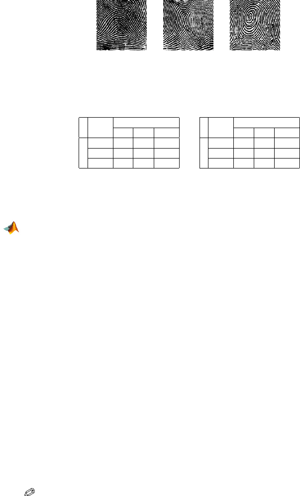
Example 14.4. Galton and ALW Features in Fingerprints. In his inﬂuen-

tial book Finger Prints, Sir Francis Galton details the description and distri-

butions of arch-loop-whorl (ALW) features of human ﬁngerprints (Fig. 14.1).

Some of his ﬁndings from 1892 are still in use today.

Tables 14.1a,b are from Galton (1892) and tabulate ALW features on fore-

ﬁngers in pairs of school children.

In Table 14.1a subjects A and B are paired at random from a large pop-

ulation of subjects. In Table 14.1b, subjects A and B are two brothers with a

random assignment of order (A, B).

Galton was interested in knowing if there was any inﬂuence of fraternity

on the dependence of ALW features. Using a

-test, test for the dependence

in both tables.

: Individuals A and B are independent if characterized by their ﬁnger-

print features.

14.2 Contingency Tables: Testing for Independence 539

(a) (b) (c)

Fig. 14.1 (a) Arch, (b) loop, and (c) whorl features in a ﬁngerprint.

Table 14.1 (a) Table with random pairing of children. (b) Table with fraternal pairing.

Arch Loop Whorl

Arch 5 12 8

Loop 8 18 8

Whorl 9 20 13

Arch Loop Whorl

Arch 5 12 2

Loop 4 42 15

Whorl 1 14 10

(a) (b)

MATLAB output:

[chisq, p, expected,assoc]=tablerxc([5 12 8; 8 18 8; 9 20 13])

%(a) random pairing

%chisq = 0.6948

% p = 0.9520

% expected =

% 5.4455 12.3762 7.1782

% 7.4059 16.8317 9.7624

% 9.1485 20.7921 12.0594

% assoc =

% C: 0.0827

% V: 0.0586

[chisq, p, expected,assoc]=tablerxc([5 12 2; 4 42 15; 1 14 10])

%(b) fraternal pairing

% chisq = 11.1699

% p = 0.0247

% expected =

% 1.8095 12.3048 4.8857

% 5.8095 39.5048 15.6857

% 2.3810 16.1905 6.4286

% assoc =

% C: 0.3101

% V: 0.2306

It is evident that for random pairing, the hypothesis of independence H

not rejected (p-value 0.9520), while in the case of fraternal pairing the ﬁnger-

print features are signiﬁcantly dependent (p-value 0.0247).

Power Analysis. Power analysis for contingency tables involves evalua-

tion of a noncentral

in which the noncentrality parameter λ depends on an

appropriate effect size.