Vidakovic B. Statistics for Bioengineering Sciences: With Matlab and WinBugs Support

Подождите немного. Документ загружается.

2.5 Displaying Data 25

100

150

200

0 50 100 150 200 250

(a) (b)

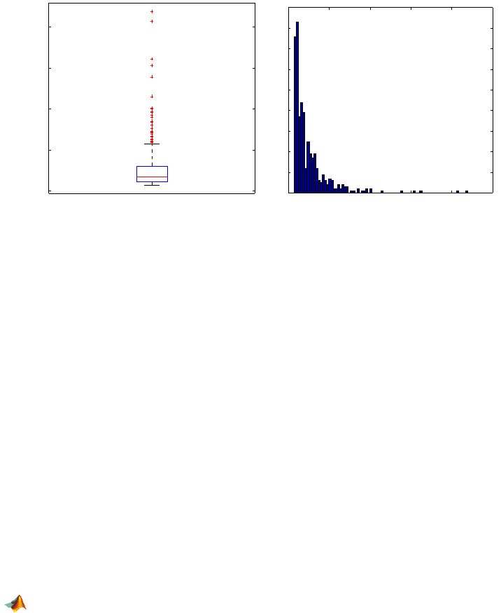
Fig. 2.4 (a) Box plot and (b) histogram of cell data

car.

For example, for cell-area data car, Sturges’ rule suggests 10 bins, Scott’s

19 bins, and the Diaconis–Freedman rule 43 bins. The default

nbins in MAT-

LAB is 10 for any sample size.

The histogram is a crude estimator of a probability density that will be dis-

cussed in detail later on (Chap. 5). A more esthetic estimator of the population

distribution is given by the kernel smoother density estimate, or

ksdensity.

We will not go into the details of kernel smoothing at this point in the text;

however, note that the spread of a kernel function (such as a Gaussian ker-

nel) regulates the degree of smoothing and in some sense is equivalent to the

choice of bin size in histograms.

Command

[f,xi,u]=ksdensity(x) computes a density estimate based on

data

x. Output f is the vector of density values evaluated at the points in xi.

The estimate is based on a normal kernel function, using a window parameter

width that depends on the number of points in x. The default width u is re-

turned as an output and can be used to tune the smoothness of the estimate,

as is done in the example below. The density is evaluated at 100 equally spaced

points that cover the range of the data in

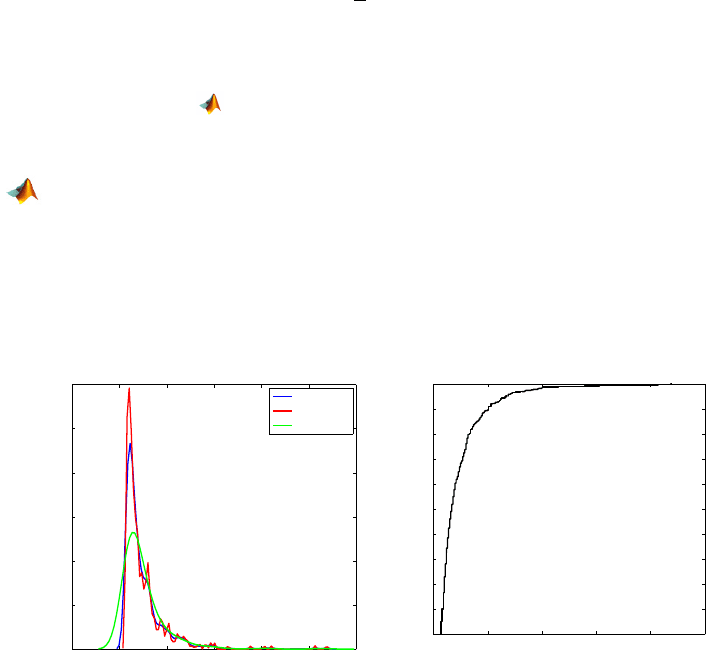
figure;

[f,x,u] = ksdensity(car);

plot(x,f)

hold on

[f,x] = ksdensity(car,’width’,u/3);

plot(x,f,’r’);

[f,x] = ksdensity(car,’width’,u

3);

plot(x,f,’g’);

legend(’default width’,’default/3’,’3

default’)

hold off

26 2 The Sample and Its Properties

Empirical Cumulative Distribution Function. The empirical cumu-

lative distribution function (ECDF) F

(x) for a sample X

,... , X

is deﬁned

(x) =

i=1

1(X

≤ x) (2.2)

and represents the proportion of sample values smaller than x. Here 1(X

≤ x)

is either 0 or 1. It is equal to 1 if

≤ x} is true, 0 otherwise.

The function

empiricalcdf(x,sample) will calculate the ECDF based on

the observations in

sample at a value x.

xx = min(car)-1:0.01:max(car)+1;

yy = empiricalcdf(xx, car);

plot(xx, yy, ’k-’,’linewidth’,2)

xlabel(’x’); ylabel(’F

n(x)’)

In MATLAB, [f xf]=ecdf(x) is used to calculate the proportion f of the

sample

x that is smaller than xf. Figure 2.5b shows the ECDF for the cell area

data,

car.

−50 0 50 100 150 200 250

0.01

0.02

0.03

0.04

0.05

0.06

default width

default/3

3 * default

0 50 100 150 200 250

0.1

0.2

0.3

0.4

0.5

0.6

0.7

0.8

0.9

(x)

(a) (b)

Fig. 2.5 (a) Smoothed histogram (density estimator) for different widths of smoothing ker-

nel; (b) Empirical CDF.

Q–Q Plots. Q–Q plots, short for quantile–quantile plots, compare the dis-

tribution of a sample with some standard theoretical distribution, such as

normal, or with a distribution of another sample. This is done by plotting the

sample quantiles of one distribution against the corresponding quantiles of the

other. If the plot is close to linear, then the distributions are close (up to a scale

2.5 Displaying Data 27

and shift). If the plot is close to the 45

◦

line, then the compared distributions

are approximately equal. In MATLAB the command

qqplot(X,Y) produces an

empirical Q–Q plot of the quantiles of the data set X vs. the quantiles of the

data set Y . If the data set Y is omitted, then

qqplot(X) plots the quantiles of

X against standard normal quantiles and essentially checks the normality of

the sample.

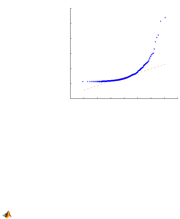
Figure 2.6 gives us the Q–Q plot of the cell area data set against the normal

distribution. Note the deviation from linearity suggesting that the distribution

is skewed. A line joining the ﬁrst and third sample quartiles is superimposed

in the plot. This line is extrapolated out to the ends of the sample to help

visually assess the linearity of the Q–Q display. Q–Q plots will be discussed in

more detail in Chap. 13.

−4 −3 −2 −1 0 1 2 3 4

−50

100

150

200

250

Standard Normal Quantiles

Quantiles of Input Sample

QQ Plot of Sample Data versus Standard Normal

Fig. 2.6 Quantiles of data plotted against corresponding normal quantiles, via qqplot.

Pie Charts. If we are interested in visualizing proportions or frequen-

cies, the pie chart is appropriate. A pie chart (

pie in MATLAB) is a graphical

display in the form of a circle where the proportions are assigned segments.

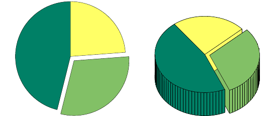
Suppose that in the cell area data set we are interested in comparing pro-

portions of cells with areas in three regions: smaller than or equal to 15, be-

tween 15 and 30, and larger than 30. We would like to emphasize the propor-

tion of cells with areas between 15 and 30. The following MATLAB code plots

the pie charts (Fig. 2.7).

n1 = sum( car <= 15 ); %n1=213

n2 = sum( (car > 15 ) & (car <= 30) ); %n2=139

n3 = sum( car > 30 ); %n3=110

28 2 The Sample and Its Properties

% n=n1+n2+n3 = 462

% proportions n1/n, n2/n, and n3/n are

% 0.4610,0.3009 and 0.2381

explode = [0 1 0]

pie([n1, n2, n3], explode)

pie3([n1, n2, n3], explode)

Note that option explode=[0 1 0] separates the second segment from the

circle. The command

pie3 plots a 3-D version of a pie chart (Fig. 2.7b).

46%

30%

24%

30%

24%

46%

(a) (b)

Fig. 2.7 Pie charts for frequencies 213, 139, and 110 of cell areas smaller than or equal to

15, between 15 and 30, and larger than 30. The proportion of cells with the area between 15

and 30 is emphasized.

2.6 Multidimensional Samples: Fisher’s Iris Data and

Body Fat Data

In the cell area example, the sample was univariate, that is, each measure-

ment was a scalar. If a measurement is a vector of data, then descriptive

statistics and graphical methods increase in importance, but they are much

more complex than in the univariate case. The methods for understanding

multivariate data range from the simple rearrangements of tables in which

raw data are tabulated, to quite sophisticated computer-intensive methods in

which exploration of the data is reminiscent of futuristic movies from space

explorations.

Multivariate data from an experiment are ﬁrst recorded in the form of ta-

bles, by either a researcher or a computer. In some cases, such tables may

appear uninformative simply because of their format of presentation. By sim-

ple rules such tables can be rearranged in more useful formats. There are

several guidelines for successful presentation of multivariate data in the form

of tables. (i) Numbers should be maximally simpliﬁed by rounding as long as

2.6 Multidimensional Samples: Fisher’s Iris Data and Body Fat Data 29

it does not affect the analysis. For example, the vector (2.1314757, 4.9956301,

6.1912772) could probably be simpliﬁed to (2.14, 5, 6.19); (ii) Organize the

numbers to compare columns rather than rows; and (iii) The user’s cognitive

load should be minimized by spacing and table lay-out so that the eye does not

travel long in making comparisons.

Fisher’s Iris Data. An example of multivariate data is provided by the cel-

ebrated Fisher’s iris data. Plants of the family Iridaceae grow on every conti-

nent except Antarctica. With a wealth of species, identiﬁcation is not simple.

Even iris experts sometimes disagree about how some ﬂowers should be classi-

ﬁed. Fisher’s (Anderson, 1935; Fisher, 1936) data set contains measurements

on three North American species of iris: Iris setosa canadensis, Iris versicolor,

and Iris virginica (Fig. 2.8a-c). The 4-dimensional measurements on each of

the species consist of sepal and petal length and width.

(a) (b) (c)

Fig. 2.8 (a) Iris setosa, C. Hensler, The Rock Garden, (b) Iris virginica, and (c) Iris versicolor,

(b) and (c) are photos by D. Kramb, SIGNA.

The data set fisheriris is part of the MATLAB distribution and contains

two ﬁles:

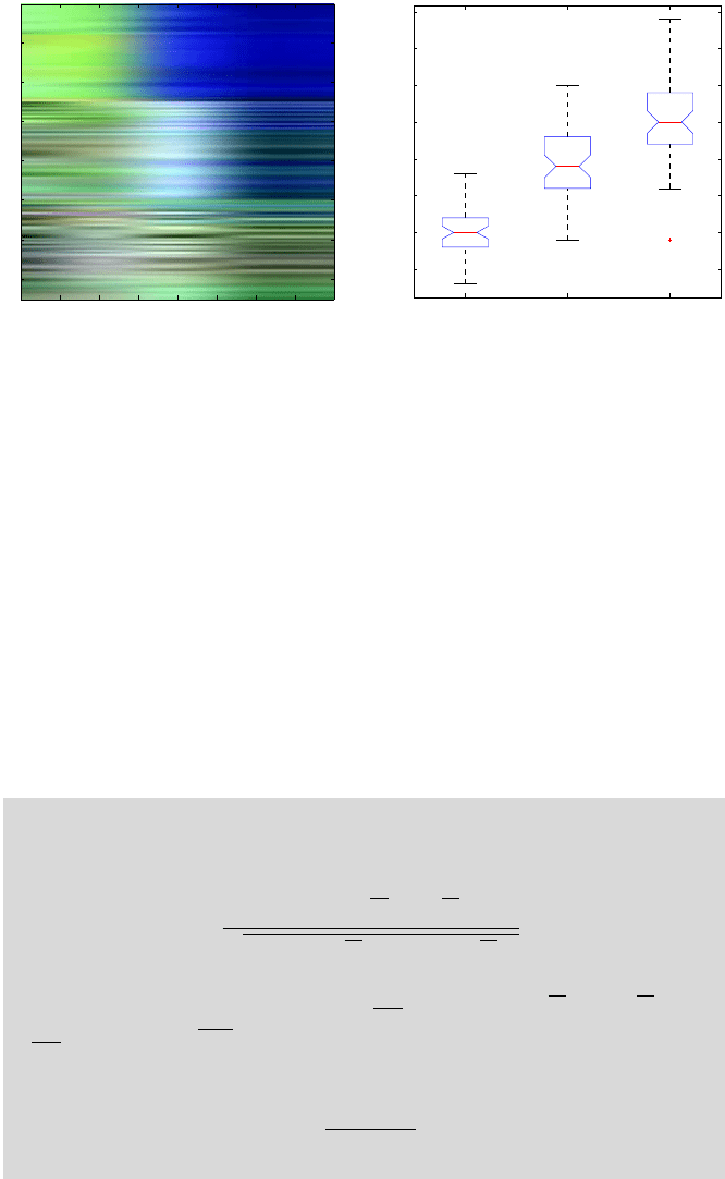
meas and species. The meas ﬁle, shown in Fig. 2.9a, is a 150 ×4

matrix and contains 150 entries, 50 for each species. Each row in the matrix

meas contains four elements: sepal length, sepal width, petal length, and petal

width. Note that the convention in MATLAB is to store variables as columns

and observations as rows.

The data set

species contains names of species for the 150 measurements.

The following MATLAB commands plot the data and compare sepal lengths

among the three species.

load fisheriris

s1 = meas(1:50, 1); %setosa, sepal length

s2 = meas(51:100, 1); %versicolor, sepal length

s3 = meas(101:150, 1); %virginica, sepal length

s = [s1 s2 s3];

figure;

imagesc(meas)

30 2 The Sample and Its Properties

0.5 1 1.5 2 2.5 3 3.5 4 4.5

100

120

140

setosa versicolor virginica

4.5

5.5

6.5

7.5

Values

(a) (b)

Fig. 2.9 (a) Matrix

meas in fisheriris, (b) Box plots of Sepal Length (the ﬁrst column in

matrix

meas) versus species.

figure;

boxplot(s,’notch’,’on’,...

’labels’,{’setosa’,’versicolor’,’virginica’})

Correlation in Paired Samples. We will brieﬂy describe how to ﬁnd the cor-

relation between two aligned vectors, leaving detailed coverage of correlation

theory to Chap. 15.

Sample correlation coefﬁcient r measures the strength and direction of

the linear relationship between two paired samples X

= (X

, X

,... , X

) and

= (Y

,... , Y

). Note that the order of components is important and the

samples cannot be independently permuted if the correlation is of inter-

est. Thus the two samples can be thought of as a single bivariate sample

), i =1, . .., n.

The correlation coefﬁcient between samples X =(X

, X

,... , X

) and Y =

,... , Y

) is

−X )(Y

−Y )

−X )

−Y )

The summary

Cov(X ,Y ) =

n−1

− X )(Y

− Y ) =

n−1

−nX Y

is called the sample covariance. The corre-

lation coefﬁcient can be expressed as a ratio:

ov(X ,Y )

2.6 Multidimensional Samples: Fisher’s Iris Data and Body Fat Data 31

where s

and s

are sample standard deviations of samples X and Y .

Covariances and correlations are basic exploratory summaries for paired

samples and multivariate data. Typically they are assessed in data screening

before building a statistical model and conducting an inference. The correla-

tion ranges between –1 and 1, which are the two ideal cases of decreasing and

increasing linear trends. Zero correlation does not, in general, imply indepen-

dence but signiﬁes the lack of any linear relationship between samples.

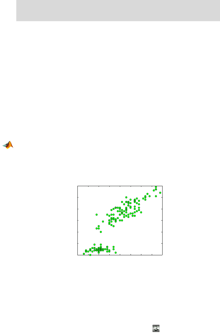
To illustrate the above principles, we ﬁnd covariance and correlation be-

tween sepal and petal lengths in Fisher’s iris data. These two variables cor-

respond to the ﬁrst and third columns in the data matrix. The conclusion is

that these two lengths exhibit a high degree of linear dependence as evident

in Fig. 2.10. The covariance of 1.2743 by itself is not a good indicator of this

relationship since it is scale (magnitude) dependent. However, the correlation

coefﬁcient is not inﬂuenced by a linear transformation of the data and in this

case shows a strong positive relationship between the variables.

load fisheriris

X = meas(:, 1); %sepal length

Y = meas(:, 3); %petal length

cv = cov(X, Y); cv(1,2) %1.2743

r = corr(X, Y) %0.8718

4 4.5 5 5.5 6 6.5 7 7.5 8

Fig. 2.10 Correlation between petal and sepal lengths (columns 1 and 3) in iris data set.

Note the strong linear dependence with a positive trend. This is reﬂected by a covariance of

1.2743 and a correlation coefﬁcient of 0.8718.

In the next section we will describe an interesting multivariate data set

and, using MATLAB, ﬁnd some numerical and graphical summaries.

Example 2.4. Body Fat Data. We also discuss a multivariate data set an-

alyzed in Johnson (1996) that was submitted to

http://www.amstat.

32 2 The Sample and Its Properties

Fig. 2.11 Water test to determine body density. It is based on underwater weighing

(Archimedes’ principle) and is regarded as the gold standard for body composition assess-

ment.

Percentage of body fat, age, weight, height, and ten body circumference

measurements (e.g., abdomen) were recorded for 252 men. Percent of body fat

is estimated through an underwater weighing technique (Fig. 2.11).

The data set has 252 observations and 19 variables. Brozek and Siri in-

dices (Brozek et al., 1963; Siri, 1961) and fat-free weight are obtained by the

underwater weighing while other anthropometric variables are obtained using

scales and a measuring tape. These anthropometric variables are less intru-

sive but also less reliable in assessing the body fat index.

– Variable description

3–5 casen Case number

10–13 broz Percent body fat using Brozek’s equation: 457/density – 414.2

18–21 siri Percent body fat using Siri’s equation: 495/density – 450

24–29 densi Density (gm/cm

)

36–37 age Age (years)

40–45 weight Weight (lb.)

49–53 height Height (in.)

58–61 adiposi Adiposity index = weight/(height

) (kg/m

)

65–69 ffwei Fat-free weight = (1 – fraction of body fat) × weight, using Brozek’s

formula (lb.)

74–77 neck Neck circumference (cm)

81–85 chest Chest circumference (cm)

89–93 abdomen Abdomen circumference (cm)

97–101 hip Hip circumference (cm)

106–109 thigh Thigh circumference (cm)

114–117 knee Knee circumference (cm)

122–125 ankle Ankle circumference (cm)

130–133 biceps Extended biceps circumference (cm)

138–141 forearm Forearm circumference (cm)

146–149 wrist Wrist circumference (cm) “distal to the styloid processes”

Remark: There are a few false recordings. The body densities for cases 48,

76, and 96, for instance, each seem to have one digit in error as seen from

org/publications/jse/datasets/fat.txt and featured in Penrose et al.

(1985). This data set can be found on the book’s Web page as well, as

fat.dat.

2.7 Multivariate Samples and Their Summaries* 33

the two body fat percentage values. Also note the presence of a man (case 42)

over 200 lb. in weight who is less than 3 ft. tall (the height should presumably

be 69.5 in., not 29.5 in.)! The percent body fat estimates are truncated to zero

when negative (case 182).

load(’\your path\fat.dat’)

casen = fat(:,1);

broz = fat(:,2);

siri = fat(:,3);

densi = fat(:,4);

age = fat(:,5);

weight = fat(:,6);

height = fat(:,7);

adiposi = fat(:,8);

ffwei = fat(:,9);

neck = fat(:,10);

chest = fat(:,11);

abdomen = fat(:,12);

hip = fat(:,13);

thigh = fat(:,14);

knee = fat(:,15);

ankle = fat(:,16);

biceps = fat(:,17);

forearm = fat(:,18);

wrist = fat(:,19);

We will further analyze this data set in this chapter, as well as in Chap. 16,

in the context of multivariate regression.

2.7 Multivariate Samples and Their Summaries*

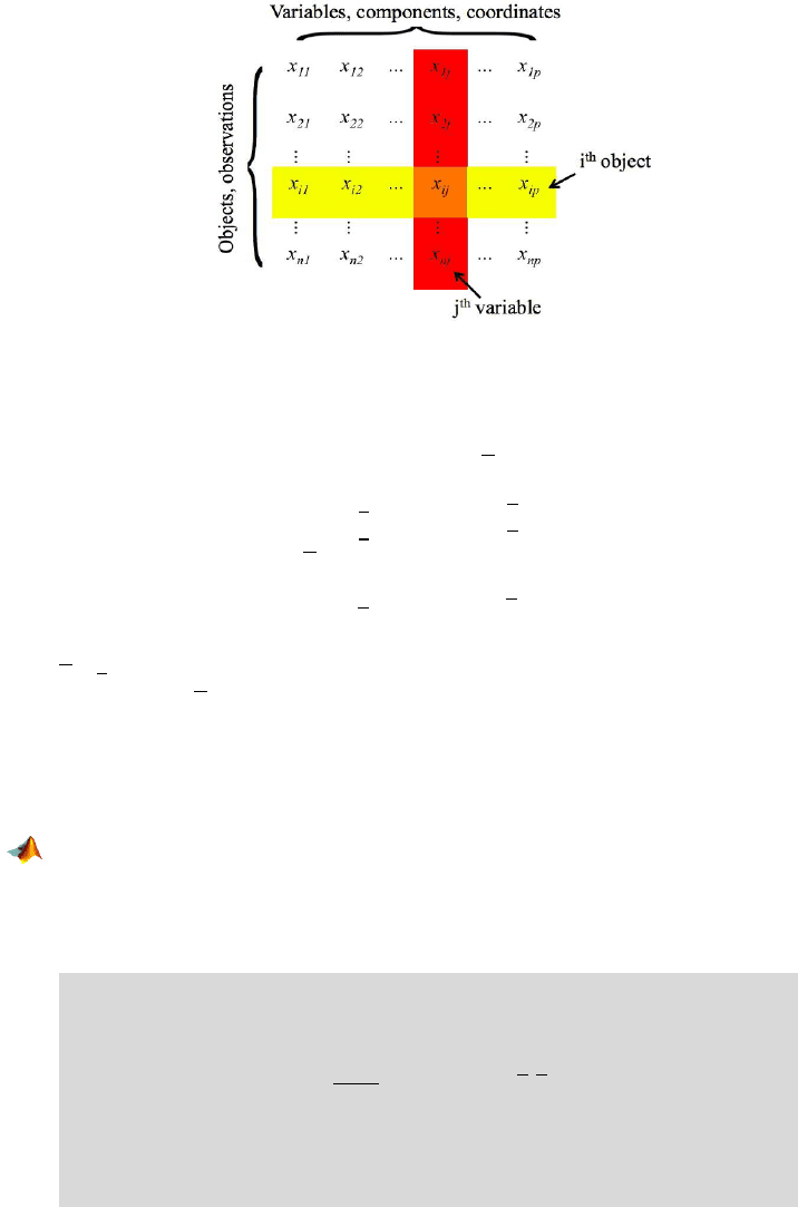
Multivariate samples are organized as a data matrix, where the rows are ob-

servations and the columns are variables or components. One such data ma-

trix of size n

× p is shown in Fig. 2.12.

The measurement x

i j

denotes the jth component of the ith observation.

There are n row vectors x

, x

,..., x

and p columns x

(1)

, x

(2)

,..., x

(n)

, so

that













(1)

, x

(2)

,... , x

(n)

Note that x

= (x

, x

,... , x

i p

)

is a p-vector denoting the ith observation,

while x

( j)

= (x

1 j

, x

2 j

,... , x

n j

)

is an n-vector denoting values of the jth vari-

able/component.

34 2 The Sample and Its Properties

Fig. 2.12 Data matrix X . In the multivariate sample the rows are observations and the

columns are variables.

The mean of data matrix X is a vector x, which is a p-vector of column

means

x =







i p



















By denoting a vector of ones of size n

×1 as 1, the mean can be written as

x =

·1, where X

is the transpose of X.

Note that

x is a column vector, while MATLAB’s command mean(X) will

produce a row vector. It is instructive to take a simple data matrix and in-

spect step by step how MATLAB calculates the multivariate summaries. For

instance,

X = [1 2 3; 4 5 6];

[n p]=size(X) %[2 3]: two 3-dimensional observations

meanX = mean(X)’ %or mean(X,1), along dimension 1

%transpose of meanX needed to be a column vector

meanX = 1/n

X’

ones(n,1)

For any two variables (columns) in X , x

(i)

and x

( j)

, one can ﬁnd the sam-

ple covariance:

i j

n −1

k=1

k j

−nx

All s

i j

s form a p × p matrix, called a sample covariance matrix and de-

noted by S.