Vidakovic B. Statistics for Bioengineering Sciences: With Matlab and WinBugs Support

Подождите немного. Документ загружается.

7.4 Conﬁdence Intervals 257

% Clopper-Pearson Intervals

Fs = finv(0.975, 2

(n-X1 + 1), 2

X1);

Fss = finv(0.975, 2

(X1+1), 2

(n-X1));

CP3 = [ X1/(X1 + (n-X1+1).

Fs), ...

(X1+1).

Fss./(n - X1 + (X1+1).

Fss)];

Fs = finv(0.975, 2

(n-X2 + 1), 2

X2);

Fss = finv(0.975, 2

(X2+1), 2

(n-X2));

CP6 = [ X2/(X2 + (n-X2+1).

Fs), ...

(X2+1).

Fss./(n - X2 + (X2+1).

Fss)];

%CP3 = 0.421 0.75246

%CP6 = 0.079621 0.35155

%==========================================

% Anscombe ARCSIN intervals

p1h = (X1 + 3/8)/(n + 3/4); p2h = (X2 + 3/8)/(n + 3/4);

AA3 = [(sin(asin(sqrt(p1h))-norminv(0.975)/(2

sqrt(n))))^2, ...

(sin(asin(sqrt(p1h))+norminv(0.975)/(2

sqrt(n))))^2];

AA6 = [(sin(asin(sqrt(p2h))-norminv(0.975)/(2

sqrt(n))))^2, ...

(sin(asin(sqrt(p2h))+norminv(0.975)/(2

sqrt(n))))^2];

%AA3 = 0.43235 0.74353

%AA6 = 0.085489 0.3366

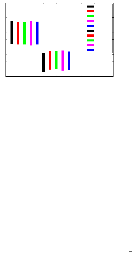
Figure 7.9 shows the pairs of conﬁdence intervals at the 3- and 6-month

follow-ups. Wald’s intervals are in black, Wilson’s in red, the Wilson score in

green, Clopper–Pearson’s in magenta, and ArcSin in blue. Notice that for all

methods, the conﬁdence intervals at the 3- and 6-month follow-ups are well

separated, suggesting a signiﬁcant change in the proportions. There are differ-

ences among the intervals, in their centers and lengths, for a particular time

of follow-up. However, as Fig. 7.9 indicates, these differences are not large.

How does one ﬁnd the conﬁdence interval for the probability of success if

in n trials no successes have been observed?

7.4.4 Conﬁdence Intervals for Proportions When X =0

When the binomial probability is small, then it is not unusual that out of n tri-

als no successes have been observed. How do we ﬁnd a (1

−α)100% conﬁdence

interval in such a case? The Clopper–Pearson interval is possible for X

= 0,

and it is given by [0,1

−(α/2)

1/n

An alternative interval can be established from the following considera-

tion. Note that (1

− p)

is the probability of no success in n trials, and this

probability is at least

α:

− p)

≥α.

258 7 Point and Interval Estimators

0 2 4 6 8 10 12 14 16

0.1

0.2

0.3

0.4

0.5

0.6

0.7

0.8

0.9

3 month follow−up

6 month follow−up

1:Wald

2:Wilson

3:WScore

4:Clopper

5:ArcSin

6:Wald

7:Wilson

8:WScore

9:Clopper

10:ArcSin

Fig. 7.9 Conﬁdence intervals at 3- and 6-month follow-ups. Wald’s intervals are in black,

Wilson’s in red, the Wilson Score in green, Clopper–Pearson’s in magenta, and ArcSin in

blue.

Since n log(1 − p) ≥log(α) and log(1 − p) ≈−p, then

≤−log(α)/n.

This is a basis for the so-called 3/n rule: 95% conﬁdence interval for p is [0, 3/n]

if no successes have been observed since

−log(0.05) = 2.9957 ≈ 3. By symme-

try, the 95% conﬁdence interval for p when n successes are observed in n

experiments is [1

−3/n,1]. When n is small, this rule leads to intervals that

are too wide to be useful. See Exercise 7.29 for a comparison of the Clopper–

Pearson and 3/n-rule intervals. We will argue in the next chapter that in the

case where no successes are observed, one should approach the inference in a

Bayesian manner.

7.4.5 Designing the Sample Size with Conﬁdence Intervals

In all previous examples it was assumed that we had data in hand. Thus,

we looked at the data after the sampling procedure had been completed. It

is often the case that we have control over what sample size to adopt before

the sampling. How large should the sample be? A sample that is too small

may affect the validity of our statistical conclusions. On the other hand, an

unnecessarily large sample wastes money, time, and resources.

The length L of the (1

−α)100% conﬁdence interval is L =2z

1−α/2

σ/

n for

the normal mean and L

= 2z

1−α/2

p(1

−

p)/n for the population proportion.

7.4 Conﬁdence Intervals 259

The sample size n is determined by solving the above equations when L is

ﬁxed.

(i) Sample size for estimating the mean: σ

is known:

≥

−α/2

where L is the length of the interval.

(ii) Sample size for estimating the proportion:

≥

−α/2

p(1

−

where

p is the sample proportion.

Designing the sample size usually precedes the sampling. In the ab-

sence of data,

p is our best guess. In the absence of any information, the

most conservative choice is

=0.5.

It is possible to express L

in the units of variance of observations, σ

, for

the normal and p(1

− p) for the Bernoulli distribution. Therefore, it is sufﬁ-

cient to state that L/

σ is 1/2, for example, or that L/

p(1 − p) is 1/4, and the

required sample size can be calculated.

Example 7.11. Cholesterol Level. Suppose you are designing a cholesterol

study experiment and would like to estimate the mean cholesterol level of all

students on a large metropolitan campus. You plan to take a random sample of

n students and measure their cholesterol levels. Previous studies have shown

that the standard deviation is 25, and you intend to use this value in planning

your study.

If a 99% conﬁdence interval with a total length not exceeding 12 is desired,

how many students should you include in your sample?

Sol. For a 99% conﬁdence level, the normal 0.995 quantile is needed, z

0.995

2.58. Then, n ≥

4·2.5758

·25

= 115.1892, and the sample size is 116 since

115.1892 should be rounded to the closest larger integer.

The margin of error is deﬁned as half of the length of a 95% conﬁdence interval

for unknown proportion, location, scale, or some other population parameter

of interest.

In popular use, however, margin of error is usually connected with public

opinion polls and represents the quantiﬁable sampling error built into well-

260 7 Point and Interval Estimators

designed sampling schemes. For estimating the true proportion of voters fa-

voring a particular candidate, an approximate 95% conﬁdence interval is

−1.96

q/n,

+1.96

q/n

where

p is the sample proportion of voters favoring the candidate,

= 1 −

1.96 is the normal 97.5 percentile, and n is the sample size. Since

≤ 1/4,

the margin of error, 1.96

q/n, is usually conservatively rounded to

For example, if a survey of n

=1600 voters yields that 52% favor a particu-

lar candidate, then the margin of error can be estimated as 1/

1600 = 1/40 =

0.025 =2.5% and is independent of the realized proportion of 52%.

However, if the true proportion is not close to 1/2, the precision of the mar-

gin of error can be improved by selecting a less conservative upper bound on

q. For example, if a survey of n

= 1600 citizens yields that 16% of them fa-

vor policy P, the margin of error can be estimated as 1.96

0.2 ·0.8/1600 ≈

1/50 = 0.02 = 2% if we are sure that the true proportion of citizens supporting

policy P does not exceed 20%.

7.5 Prediction and Tolerance Intervals*

In addition to conﬁdence intervals for the parameters, a researcher may be

interested in predicting future observations. This leads to prediction intervals.

We will exemplify the prediction interval for predicting future observations

from a normal population

N (µ,σ

) once X

,... , X

have been observed. De-

note the future observation by X

n+1

Consider

X and X

n+1

. These two random variables are independent and

their difference has a normal distribution,

X −X

n+1

∼N (0,σ

/n +σ

thus, Z

X −X

n+1

1+1/n

has a standard normal distribution. This leads to (1−α)100%

prediction intervals for X

n+1

If σ

is known, then

X −z

1−α/2

1 +

X +z

1−α/2

1 +

is not known, then

7.5 Prediction and Tolerance Intervals* 261

X −t

n−1,1−α/2

1 +

X +t

n−1,1−α/2

1 +

Note that prediction intervals contain the factor

1 +

in place of

in matching conﬁdence intervals for the normal population mean. When n is

large, the prediction interval can be substantially larger than the conﬁdence

interval. This is because the uncertainty about the future observation has two

parts: (1) uncertainty about its mean plus (2) uncertainty about the individual

response.

Tolerance intervals place bounds on ﬁxed portions of population distribu-

tions with a speciﬁed conﬁdence. For example, the question What interval will

contain 95% of the population measurements with 99% conﬁdence? is answered

by a tolerance interval. The ends of a tolerance interval are called tolerance

limits. A manufacturer of medical devices might be interested in the propor-

tion of production for which a particular dimension falls within a given range.

For normal populations, the two-sided interval is deﬁned as

[X −ks, X +ks], k =

−1) z

−γ/2

n χ

−1,α

(7.8)

and interpreted as follows. With a conﬁdence of 1

−α, the proportion of 1 −γ

of population measurements will fall between the lower and upper bounds in

(7.8).

Example 7.12. For sample size n

=20, X = 12, s =0.1, conﬁdence 1 −α = 99%,

and proportion 1

−γ = 95%, the tolerance factor k is calculated as in the fol-

lowing MATLAB script:

n=20;

z = norminv(1-0.05/2) %proportion of 1-0.05=0.95

%z = 1.9600

xi = chi2inv(0.01, n-1) %confidence 1-0.01=0.99

%xi = 7.6327

k = sqrt( (n^2-1)

z^2/(n

xi) )

%k = 3.1687

[12-k

0.1 12+k

0.1]

%11.6831 12.3169

262 7 Point and Interval Estimators

and the tolerance interval is [11.6831,12.3169].

7.6 Conﬁdence Intervals for Quantiles*

The conﬁdence interval for a normal quantile is based on a noncentral t dis-

tribution. Let X

,... , X

be a sample of size n with the sample mean X and

sample standard deviation s.

It is of interest to ﬁnd a conﬁdence interval on the population’s pth quan-

tile,

µ +z

×σ, with a conﬁdence level of 1 −α.

The conﬁdence interval is given by [L,U], where

= X +s ·nct(α/2,n −1,

n ·z

= X +s ·nct(1−α/2, n −1

n ·z

and nct(q,d f , nc) is the q-quantile of the noncentral t distribution (p. 217)

with d f the degrees of freedom and noncentrality parameter nc.

The conﬁdence intervals for quantiles can be based on order statistics when

normality is not assumed. For example, instead of declaring the conﬁdence

interval for the mean, one should report the conﬁdence interval on the median

if the normality of the data is a concern. Let X

(1)

, X

(2)

,... , X

(n)

be the order

statistics of the sample. Then a (1

−α)100% conﬁdence interval for the median

Me is

(h)

≤ M e ≤ X

(n−h+1)

The value of h is usually given by tables. For large n (n

>40) a good approxi-

mation for h is an integer part of

−z

1−α/2

n −1

As an illustration, if n

=300, the 95% conﬁdence interval for the median is

(132)

, X

(169)

] since

n = 300;

h = floor( (n - 1.96

sqrt(n) - 1)/2 )

% h = 132

n - h + 1

% ans = 169

7.7 Conﬁdence Intervals for the Poisson Rate* 263

7.7 Conﬁdence Intervals for the Poisson Rate*

Recall that an observation X coming from P oi(λ) has both a mean and a vari-

ance equal to the rate parameter,

EX = Var X = λ, and that Poisson random

variables are “additive in the rate parameter”:

, X

,... , X

∼P oi(λ) ⇒ nX =

i=1

∼P oi(nλ). (7.9)

The asymptotically shortest Wald-type (1

−α)100% interval for λ is ob-

tained using the fact that Z

(X −λ) is approximately the standard nor-

mal. The inequality

|X −λ| ≤ z

1−α/2

leads to

−λ

2X +

−α/2

(X )

≤ 0,

which solves to





X +

−α/2

−z

1−α/2

−α/2

, X +

−α/2

1−α/2

−α/2





Other Wald-type intervals are derived from the fact that

X −

1/(4n)

is approx-

imately the standard normal. Variance stabilizing, modiﬁed variance stabiliz-

ing, and recentered variance stabilizing (1

−α)100% conﬁdence intervals are

given as (Barker, 2002)





X −z

1−α/2

X +z

1−α/2









X +

−α/2

−z

1−α/2

X +

−α/2

1−α/2









X +

−α/2

−z

1−α/2

X +3/8

X +

−α/2

1−α/2

X +3/8





An alternative approach is based on the link between Poisson and

dis-

tributions. Namely, if X

∼P oi(λ), then

264 7 Point and Interval Estimators

P(X > x) =P(Y <2λ), for Y ∼χ

and the (1 −α)100% conﬁdence interval for λ when X is observed is

2X ,

α/2

2(X

+1),1−α/2

where

2X ,

α/2

and χ

2(X

+1),1−α/2

are α/2 and 1 −α/2 quantiles of the χ

dis-

tribution with 2X and 2(X

+1) degrees of freedom, respectively. Due to the

additivity property (7.9), the conﬁdence interval changes slightly for the case

of an observed sample of size n, X

, X

,... , X

. One ﬁnds S =

, which is

a Poisson with parameter n

λ and proceeds as in the single-observation case.

The interval obtained is for n

λ and the bounds should be divided by n to get

the interval for

λ:

2S,

α/2

2(S

+1),1−α/2

Example 7.13. Counts of

α-Particles. Rutherford et al. (1930, pp. 171–172)

provide descriptions and data on an experiment by Rutherford and Geiger

(1910) on the collision of

α-particles emitted from a small bar of polonium with

a small screen placed at a short distance from the bar. The number of such

collisions in each of 2608 eight-minute intervals was recorded. The distance

between the bar and screen was gradually decreased so as to compensate for

the decay of radioactive substance.

X 0 1 2 3 4 5 6 7 8 9 10 11 ≥12

Frequency

57 203 383 525 532 408 273 139 45 27 10 4 2

It is postulated that because of the large number of atoms in the bar and

the small probability of any of them emitting a particle, the observed frequen-

cies should be well modeled by a Poisson distribution.

%Rutherford.m

X=[ 0 1 2 3 4 5 6 7 8 9 10 11 12 ];

fr=[ 57 203 383 525 532 408 273 139 45 27 10 4 2];

n = sum(fr); %number of experiments//time intervals

rfr = fr./n; %relative frequencies %n=2608

xbar = X

rfr’ ; %lambdahat = xbar = 3.8704

tc = X

fr’; %total number of counts tc = 10094

%Recentered Variance Stabilizing

[xbar + (norminv(0.975))^2/(4

n) - ...

norminv(0.975)

sqrt(( xbar + 3/8)/n )...

xbar + (norminv(0.975))^2/(4

n) + ...

norminv(0.975)

sqrt( (xbar+ 3/8)/n )]

% 3.7917 3.9498

% Poisson/Chi2 link

[1/(2

chi2inv(0.025, 2

tc) ...

1/(2

chi2inv(0.975, 2

(tc + 1))]

% 3.7953 3.9467

7.8 Exercises 265

The estimator for λ is

λ = X = 3.8704, the Wald-type recentered variance

stabilizing interval is [3.7917,3.9498], and the Pearson/chi-square link conﬁ-

dence interval is [3.7953,3.9467]. The intervals are very close to each other

and quite tight due to the large sample size.

Sample Size for Estimating λ. Assume that we are interested in esti-

mating the Poisson rate parameter

λ from the sample X

,... , X

. Chen (2008)

provided a simple way of ﬁnding the sample size n necessary for

λ =

to satisfy

λ −λ|<²

} or {|

λ/λ −1|<²

}) >1 −δ

for δ,²

, and ²

small. The minimal sample size is

n >

ln2 −lnδ

(1 +²

)ln(1 +²

) −²

For example, the sample size needed to ensure that the absolute error is

less than 0.5 or that the relative error is less than 5% with a probability of

0.99 is n

=431.

delta = 0.01; epsa =0.5; epsr = 0.05;

n = epsr/epsa

log(2/delta)/((1+epsr)

log(1+epsr)-epsr)

% n = 430.8723

Note that both tolerable relative and absolute errors, ²

and ²

, need to be

speciﬁed since the precision criterion involves the probability of a union.

7.8 Exercises

7.1. Tricky Estimation. A publisher gives the proofs of a new book to two

different proofreaders, who read it separately and independently. The ﬁrst

proofreader found 60 misprints, the second proofreader found 70 misprints,

and 50 misprints were found by both. Estimate how many misprints remain

undetected in the book?

Hint:

Refer to Example 5.10.

7.2. Laplace’s Rule of Succession. Laplace’s Rule of Succession states that if

an event appeared X times out of n trials, the probability that it will appear

in a future trial is

X +1

n+2

266 7 Point and Interval Estimators

(a) If

X +1

n+2

is taken as an estimator for binomial p, compare the MSE of this

estimator with the MSE of the traditional estimator,

(b) Represent MSE from (a) as the sum of the estimator’s variance and the

bias squared.

7.3. Neurons Fire in Potter’s Lab. The data set

neuronfires.mat was

compiled by student Ravi Patel while working in Professor Steve Potter’s

lab at Georgia Tech. It consists of 989 ﬁring times of a cell culture of neu-

rons. The recorded ﬁring times are time instances when a neuron sent a

signal to another linked neuron (a spike). The cells, from the cortex of an

embryonic rat brain, were cultured for 18 days on multielectrode arrays.

The measurements were taken while the culture was stimulated at the

rate of 1 Hz. It was postulated that ﬁring times form a Poisson process;

thus interspike intervals should have an exponential distribution.

(a) Calculate the interspike intervals T using MATLAB’s

diff command.

Check the histogram for T and discuss its resemblance to the exponential

density. By the moment matching estimator argue that exponential param-

eter

λ is close to 1.

(b) According to (a), the model for interspike intervals is T

∼ E (1). You are

interested in the proportion of intervals that are shorter than 3, T

≤3. Find

this proportion from the theoretical model

E (1) and compare it to the esti-

mate from the data. For the theoretical model, use

expcdf and for empirical

data use

sum(T <= 3)/length(T).

–1 0 1

Prob θ 2θ 1 −3θ

(a) What is the possible range for θ?

(b) What is the MLE for

θ.

7.5. MLE for Two Continuous Distributions. Find the MLE for parameter

θ if the model for observations X

, X

,... , X

, is

(a) f (x

|θ) =

, 0 <θ ≤ x;

(b) f (x

|θ) =

θ −1

, x ≥1, θ >1.

7.6. Match the Moment. The geometric distribution (X is the number of fail-

ures before the ﬁrst success) has a probability mass function of

f (x

|p) = q

p, x =0, 1, 2,....

7.4. The MLE in a Discrete Case.A sample

−1,1,1,0, −1, 1,1,1,0,1,1,0,−1,1,1

was observed from a population with a probability mass function of