Stevenson J. Power system analysis
Подождите немного. Документ загружается.

346 CHAPTER 9 POWER·FLOW SOLUTIONS
and updating the jacobian, we compute the new corrections
[aX�l) 1
=
[
3.658453
a X�l)
-
0.552921
- 0.597753
]
-1
[ -0.047079
]
=
[-0.016335 ]
3.444916 - 0.064047 - 0.021214
These corrections also exceed the precision index, and so we move on to the
next iteration with the new corrected values
X
�
2
) = -0.150 +
(
- 0.01(335)
=
-0.166335 rad
x�
2
)
=
0.925 +
(
-0.021214)
=
0.903786
Continuing on to the third iteration, we nd that the corrections x\
J
) and
ax�3) are each smaller in magnitude than the stipulated tolerance of 10
-5
.
Accordingly, we calculate the solution
X\4)
=
-0.166876 rad;
X�
4
)
=
0.903057
The resultant mismatches are insignicant as may be easily checked.
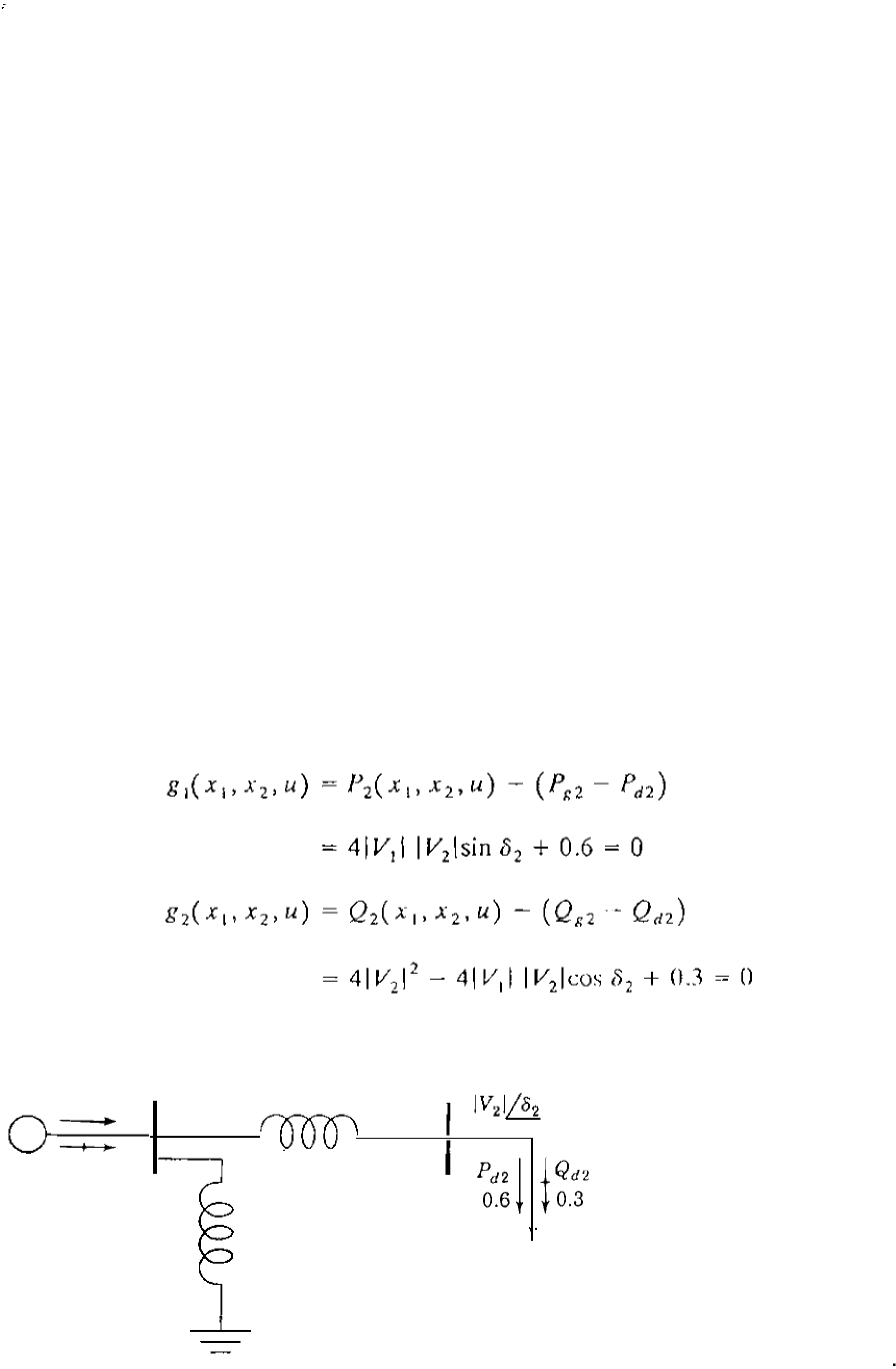
In this example we have actually solved our rst power-ow problem by
the Newton-Raphson method. This is because the two nonlinear equations of
the example are the power-ow equations for the simple system shown in
Fig. 9.3,
Pg1
I
V
ll!
-
Qg
l
)6.0
®
)0.25
To load
(9.36)
(
9.37)
GURE 9
The system with power-ow
equations corresponding to
those of Example 9.4.
9.4
THE NEWTON-RAPHSON POWER-FLOW SOLUTION
347
where x
I
represents the angle O
2
and x 2 represents the vol tage magnitude I
V
21
at bus
. The control u denotes the voltage
magnitude
I
V
I
I
o
f the slack bus,
and by changing its value from the specied value of 1.0 per unit, we may
control the solution to the problem. In this textbook we do not investigate this
control characteristic but, rather, concentrate on the application of the
Newton-Raphson procedure in power-flow studies.
9.4 THE NEWTON-RAPHSON POWER-FLOW
SOLUTION
To apply the Newton-Rap hson met hod to the so lution of the power-ow
equat ions, we express bus voltages and line admittances in polar form. When n
is set equal to i in ES. (9.6) and (9.7) ancl the corresponding terms are
scr;lratc rrom t hc SUm;l{ ions, wc obt<lin
/J;
=
I
�f (;u +
L I
V
i
- 2008 — 2025 «СтудМед»