Stefanica D. A Primer for the Mathematics of Financial Engineering
Подождите немного. Документ загружается.

44
CHAPTER
1.
CALCULUS
REVIEW.
OPTIONS.
• Portfolio
2:
Long two call
options
with
strike K =
X?
(All options
are
on
the
same
asset
and
have
the
same
maturity.)
14. Call options
with
strikes 100, 120,
and
130
on
the
same
underlying asset
and
with
the
same
maturity
are
trading
for 8, 5,
and
3, respectively
(there
is no
bid-ask
spread).
Is
there
an
arbitrage
opportunity
present?
If
yes, how
can
you
make
a riskless profit?
15. A
stock
with
spot
price 40
pays
dividends continuously
at
a
rate
of
3%.
The
four
months
at-the-money
put
and
call options
on
this
asset
are
trading
at
$2
and
$4, respectively.
The
risk-free
rate
is
constant
and
equal
to
5%
for all times. Show
that
the
Put-Call
parity
is
not
satisfied
and
explain how would
you
take
advantage of
this
arbitrage
opportunity.
16.
The
bid
and
ask
prices for a six
months
European
call
option
with
strike
40
on
a
non-dividend-paying
stock
with
spot
price 42
are
$5
and
$5.5,
respectively.
The
bid
and
ask
prices for a six
months
European
put
option
with
strike 40
on
the
same
underlying asset
are
$2.75
and
$3.25,
respectively. Assume
that
the
risk free
rate
is equal
to
O.
Is
there
an
arbitrage
opportunity
present?
17. You
expect
that
an
asset
with
spot
price $35 will
trade
in
the
$40-$45
range
in
one year.
One
year
at-the-money
calls
on
the
asset
can
be
bought
for $4. To
act
on
the
expected
stock
price appreciation, you
decide
to
either
buy
the
asset,
or
to
buy
ATM calls.
Which
strategy
is
better,
depending
on
where
the
asset price will
be
in
a year?
18.
The
risk free
rate
is 8%
compounded
continuously
and
the
dividend
yield
of
a stock
index
is 3%.
The
index
is
at
12,000
and
the
futures
price
of
a
contract
deliverable
in
three
months
is 12,100. Is
there
an
arbitrage
opportunity,
and
how do
you
take
advantage
of
it?
Chapter
2
Improper
integrals.
Numerical
integration.
Interest
rates.
Bonds.
Double integrals. Switching
the
order
of
integration.
Convergence
and
evaluation
of
improper
integrals.
Differentiating
improper
integrals
with
respect
to
the
integration
limits.
Numerical
methods
for
computing
definite integrals:
the
Midpoint, Trape-
zoidal,
and
Simpson's rules. Convergence
and
numerical implementation.
2.1
Double
integrals
Let
D C
~2
be
a
bounded
region
and
let f : D
-7
~
be
a continuous function.
The
double
integral
of
f over
D,
denoted
by
represents
the
volume
of
the
three
dimensional
body
between
the
domain
D
in
the
two dimensional plane
and
the
graph
of
the
function f (
x,
y).
The
double integral
of
f over D
can
be
computed
first
with
respect
to
the
variable
x,
and
then
with
respect
to
the
variable
y,
when
it
is denoted as
J
fv
f(x,
y)
dx
dy,
or
can
be
computed
first
with
respect
to
the
variable y,
and
then
with
respect
to
the
variable
x,
when
it
is
denoted
as
J
fv
f(x,y)
dy dx.
We will define
these
integrals
properly
in
(2.2)
and
(2.3),
and
specify
an
instance
when
the
two integrals have
the
same
value
and
are
equal
to
the
double integral
of
f over D
in
Theorem
2.1.
45
46
CHAPTER
2.
NUMERICAL
INTEGRATION.
BONDS.
For
simplicity,
assume
that
the
domain
D is
bounded
and
convex, i.e., for
any
two
points
Xl
and
X2
in
D, all
the
points
on
the
segment
joining
Xl
and
X2
are
in
D as well. Also,
assume
that
there
exist
two
continuous
functions
h(x)
and
h(x)
such
that
D
can
be
described
as
follows:
D
= {(x, y) I a
:S;
X
:S;
band
h (x)
:S;
y
:S;
h ( X
)}
• (2.1 )
The
functions h (
x)
and
h (
x)
are
well defined
by
(2.1) since
the
domain
D
is
bounded
and
convex.
Then,
by
definition,
1
r
f(x,
y) dy dx =
lb
( rh(X)
f(x,
y) d
Y
) dx. (2.2)
iD
a
ih(x)
If
there
exist two
continuous
functions
gl
(y)
and
g2
(y)
such
that
D =
{(x,
y) I c:S; y
:S;
d
and
gl(y)
:S;
x
:S;
g2(y)},
then,
by
definition,
1
r
f(x,
y) dx dy =
jd
(1
92
(Y)
f(x,
y)
dX)
dy. (2.3)
iD
c
91(Y)
Theorem
2.1.
(Fubini'
s
Theorem.)
With the notations above,
if
the
function
f(x,
y) is continuous, then the integrals (2.2) and (2.3)
are
equal
to each other and to the double integral
of
f(x,
y) over
D,
i.e., the order
of
integration
does
not
matter:
1
Ll
= 1
Ll(x,y)dXd
Y
= 1
LJ(x,y)dYdx.
For
example, if D =
[a,
b)
x
[c,
d)
is a
rectangle
and
if
f(x,
y)
is a
continuous
function,
then
1
Ll
=
lt
1
(x,Y)d
Y
dX
=
tl
1
(x,Y)dXd
Y
.
Example:
Let
D = [1,3] x [2,5]
and
f(x,
y) = 2y - 3x.
Compute
J
JD
f·
Answer: Since
f(x,
y) is
continuous,
it
follows from
Theorem
2.1
that
it
is
enough
to
compute
either
J
JD
f(x,
y)dxdy
or
J
JD
f(x,
y)dydx.
Thus,
1
Ll
[([(2
Y
-3X)dX)d
Y =
[(4
Y
-12)d
Y
=6
1 L f [
([(2
Y
-
3X)d
Y
)
dx
=
[(21-
9x)dx =
6.
D
Example:
Assume
D is a
disk
of
radius
2
centered
at
0
and
let
f (x, y) =
1 - x
2
y2.
Compute
J
JD
f·
2.1.
DOUBLE
INTEGRALS
47
Answer:
Note
that
D =
{(x,
y) : x
2
+
y2
:S;
4}.
The
points
on
the
boundary
of
D (i.e.,
on
the
circle
of
center
0
and
radius
2)
satisfy
x
2
+
y2
= 4. Solving
for
y we find
that
y2
= 4 - x
2
and
therefore y =
±.)
4 - x
2
.
This
corresponds
to
a =
-2,
b = 2,
h(x)
=
-.)4
- x
2
and
h(x)
=
.)4
- x
2
in
(2.1), i.e.,
D = { (
x,
y):
- 2
:S;
x
:S;
2
and
V 4 - x
2
:S;
Y
:S;
V 4 - x
2
}.
Then,
from
Theorem
2.1,
it
follows
that
1
r
f(x,
y) dy dx =
12
(1v'4=X2
21
- x
2
-
y2
d
Y
)
dx
iD
-2
-y4-x
1
2
((1
_ x
2
)y _
y3)
I
Y
=v'4=X2
dx
-2
3
y=-y4-x2
1
2 2(1 - x
2
)V
4 _
x2
_
2(
.J4=X2)3
dx
-2
3
-~12(1+2x2)V4-x2dX
=
_4
r\I+2X2)V4-x2dx;
3
-2
3
io
the
last
equality
follows from
Lemma
0.1, since
(1
- 2x
2
).)4 - x
2
is
an
even
function.
After
making
the
change
of
variables x = 2
sin(t),
for t E
[0,
~],
we
find
out
that
1
Ll
=
-41r.
We
note
that
this
integral
will
be
computed
in
a
more
straightforward
fashion
using
polar
coordinates;
see
section
7.2.1. 0
Let
D =
[a,
b)
x
[c,
d)
be
a
rectangle
and
let
f
(x,
y)
be
a
continuous
function
with
separated
variables, i.e.,
f(x,
y) =
g(x)h(y)
with
g(x)
and
h(y) continuous.
Then
the
two dimensional
integral
of
f(x,
y) over D is
the
product
of
two
one
dimensional
integrals:
1 L
l(x,y)
dx
dy
= t l g(x)h(y)
dx dy
= t h(y)
(l9(X)dX)
dy
=
(l
g(x) dX)
(t
h(y) dY) .
(2.4)
Note
that
this
does
not
happen
if
f(x,
y)
is
separable
but
D is
not
a
rectangle.
Let
D =
{(x,
y) : c:S; y
:S;
d,
gl(y)
:S;
x
:S;
g2(y)}
and
assume
that
f(x,
y) =
g(x)h(y).
Then,
1j
j
d192(Y)
f(x,y)
dx dy =
g(x)h(y)
dx dy
D c
~(~
48
CHAPTER
2.
NUMERICAL
INTEGRATION.
BONDS.
j
d
(j92(Y)
)
=
h(y)
g(x) dx dy.
e gl(Y)
The
integral
J~2(~)
g(x) dx is,
in
general, a function of
the
variable y. There-
fore, we
cannot
take
the
term
J~2(~)
g(
x)
dx outside
the
sign of
integration
with
respect
to
y,
as we did
in
(2.4).
2.2
Improper
integrals
We consider
three
types of
improper
integrals:
•
Integrate
the
function f (x) over
an
infinite interval of
the
form
[a,
00)
or
(-00,
b).
The
integral 1
00
f(x)
dx exists if
and
only if
the
limit as t
-----*
00
of
the
definite integral of
!(
x)
between a
and
t exists
and
is finite.
The
integral
J~oo
f (x)
dx
exists if
and
only if
the
limit as t
-----*
-00
of
the
definite integral
of
f (x) between t
and
b exists
and
is finite.
Then,
['
j(x)
dx
lim
rt
f(x)
dx;
t-+oo
Ja
(2.5)
l~
J(x) dx
lim
Ib
f(x)
dx.
t-+-oo
t
(2.6)
Adding
and
subtracting
improper
integrals of
this
type
follows rules sim-
ilar
to
those for definite integrals:
Lemma
2.1.
Let f : ~
-----*
~
be
an integrable function over the interval
[a,
00).
If
b >
a)
then
f(x)
is also integrable over the interval [b,oo) and
.r
j(x)
dx -
['
j(x)
dx = l
j(x)
dx.
Let
f(x)
be
an
integrable function over the interval
(-00,
b).
If
a <
b)
then
f(x)
is also integrable over the interval
(-00,
a)
and
l~
j(x)
dx - I:
j(x)
dx = l
j(x)
dx.
•
Integrate
the
function
f(x)
over
an
interval
[a,
b)
where
f(x)
is
unbounded
as x approaches
the
end points a
and/or
b.
For example, if
the
limit as x
~
a
2.2.
IMPROPER
INTEGRALS
49
of f (x) is infinite,
then
J:
f (x) dx exists if
and
only if
the
limit as t
~
a
of
the
definite integral of
f(x)
between t
and
b exists
and
is finite, i.e.,
r
b
f(x)
dx =
liml
b
f(x)
dx.
~
t'a
t
•
Integrate
the
function
f(x)
on
the
entire real axis, i.e.,
on
(-00,00).
The
integral
J~oo
f ( x) dx exists if
and
only if
there
exists a real
number
a such
that
both
J~oo
f(x)
dx
and
Ja
oo
f(x)
dx exist.
Then,
I:
j(x)
dx =
I:
j(x)
dx +
['
j(x)
dx (2.7)
L
a
jt2
= lim
f(x)
dx
+ lim
f(x)
dx.
t1-+-00
tl
t2-+
oo
a
(2.8)
Note
that
it
is incorrect
to
use, instead of (2.8),
the
following definition
for
the
integral
of
f(x)
over
the
real axis (-00,00):
For a simple example,
it
is easy
to
see
that
rt
x dx =
0,
V t >
0,
J-
t
(2.9)
while
J~oo
x dx =
-00
and
Jo
oo
x dx =
00,
for
any
a
E~.
Therefore, according
to
definition (2.7),
J~oo
x dx
cannot
be
defined.
However, if we know
that
the
function f (
x)
in
integrable over
the
entire
real axis,
then
we
can
use formula (2.9)
to
evaluate it:
Lemma
2.2.
If
the improper integral
J~oo
f(x)dx
exists) then
(2.10)
Example: Show
that,
for any a > 0,
(2.11)
50
CHAPTER
2.
NUMERICAL
INTEGRATION.
BONDS.
exists
and
is finite,
and
conclude
that
1
00
x2k
e
_X2
dx
-00
exists
and
is finite for
any
positive integer k. (Integrals of
this
type
need
to
be
evaluated when computing
the
expected
value
and
variance of
the
standard
normal
variable; see (3.33)
and
(3.34).)
Answer: Let h :
[0,00) ----7 R
be
given
by
h(t)
~
l'
xQe-x'
dx,
By
definition (2.5),
to
prove
that
Jo
oo
Xi:t
e
-X2
dx
exists
and
is finite,
it
is
enough
to
show
that
lim t
Xi:t
e
-X2
dx
= lim h(t)
t--+oo
J 0
t--+oo
exists
and
is finite.
(The
function
xi:t
e-X
2
is
bounded
as x
~
0 since a > 0.)
Since exponential functions increase
much
faster
than
power functions as
x goes
to
infinity,
it
follows
that
lim
Xi:t+2
e-
x2
=
O.
x--+oo
Then,
there
exists a
constant
M > 0 such
that
v
x?:
M.
For
any
t > M we
obtain
that
h(t)
~
1M
xQe'X'
dx
+ £
xQe-
X
'
dx
<
h(M)
+
£:2
dx
~
h(M)
+
(-~+
!)
1
<
h(M)
+
M'
We conclude
that
the
function h(t) is
bounded
as t ----7 00. Since h(t) is
also increasing,
it
follows
that
limt--+oo
h(
t) exists
and
is finite,
and
therefore
that
Jo
oo
xi:te-
X2
dx
exists
and
is finite.
Note
that
Jo
oo
x
2k
e-
x2
dx
exists
and
is finite;
d.
(2.11) for a = 2k.
Then,
from (5) of Lemma 0.1,
it
follows
that
2.3.
DIFFERENTIATING
IMPROPER
INTEGRALS
and
therefore
that
J~oo
x
2k
e-
x2
dx
exists
and
is finite.
Examples:
Compute
51
r
1
00
eX
dx',
r
1
1 dx'
J1
Jo
Vx
'
1
0 1
-00
(2x - 1
)3
dx;
1:
e
lxl
dx,
Answers:
1
00
e-
X
dx
1
00
eX
dx
1
1 1
-dx
oVx
1
0 1
-00
(2x -
1)3
dx
lim
rt
e-
x
dx
= lim
_e-
t
+ e-1 = 1,
t--+oo
J 1
t--+oo
e
lim r
eX
dx
= lim
eX
- e
1
= 00;
t--+oo
J 1
t--+oo
lim r
1
.
~
dx
= lim 2
2Vt
=
2;
t'\,o
Jt v x
t'\,O
lim r
O
1
dx
t--+-oo
Jt (2x - 1)3
1
1
0
lim
t--+-oo
4(2x
- 1)2 t - 4 '
1
1
0 e -ixi
dx
+
roo
e -ixi
dx
-00
Jo
1
0
eX
dx
+
roo
e-
X
dx
-00
Jo
lim r
O
eX
dx
+ lim
rz
e-
x
dx
y--+-ooJ
y
z--+ooJo
lim
eX
1
0
+ lim
(_e-
X
)
I~
y--+-oo
y
z--+oo
lim
(1
- e
Y
)
+ lim (_e-
Z
+
1)
y--+-oo
z--+oo
2.
2.3
Differentiating
improper
integrals
with
respect
to
the
integration
limits
This
topic
appears
frequently
in
conjunction
with
the
Black-Scholes pricing
model for plain vanilla options, e.g., when
exact
formulas for
the
Greeks are
computed; see Section 3.6 for more details.
52
CHAPTER
2.
NUMERICAL
INTEGRATION.
BONDS.
Lemma
2.3.
Let f :
ffi.
----7
ffi.
be
a continuous function such that the improper
integral
J~oo
f (x) dx exists. Let
g,
h :
ffi.
----7
ffi.
be
given
by
l
b(t)
g(t) =
-00
f(x)
dx;
h(t)
=
roo
f(x)
dx,
ia(t)
where a(t) and b(t)
are
differentiable functions. Then g(t) and h(t)
are
dif-
ferentiable, and
g'
(t) f(b(t))
b'
(t);
h'(t) -
f(a(t))
a'(t).
Proof.
Since
the
integral
of
f (x) over
the
entire
real axis is finite, we
can
write
the
functions g(t)
and
h(t)
as
g(t)
h(t)
=
l~
j(x)
dx +
r
O
f(x)
dx +
ia(t)
rb(t)
io
f(x)
dx;
['
j(x)
dx.
Note
that
J~oof(x)dx
and
Jo
oo
f(x)dx
are
constant
numbers whose derivative
with
respect
to
t is
O.
Then,
using
Lemma
1.2, we conclude
that
g'(t)
d (
rb(t)
)
dt
io
f(x)
dx
= f(b(t)) b'(t);
h'(t)
d
d
(rO
f(x)
dX)
t ia(t)
-
f(a(t))
a'(t).
2.4
Numerical
methods
for
computing
definite
integrals:
Midpoint
rule,
Trapezoidal
rule,
and
Simpson's
rule
o
Computing
the
value
of
a definite
integral
using
the
Fundamental
Theorem
of
Calculus is only possible if a closed formula for
the
antiderivative
of
the
function
to
integrate
can
be
obtained.
This
is
not
always possible, e.g., for
J
e-
x2
dx.
In
these cases,
approximate
values
of
the
definite
integral
are
2.4. MIDPOINT,
TRAPEZOIDAL,
AND
SIMPSON'S
RULES
53
computed
using numerical
integration
methods.
We present
three
of
the
most
common
such
methods.
Let f :
[a,
b]
----7
ffi.
be
an
integrable function. To
compute
an
approximate
value of
the
integral
1 = l
j(x)
dx,
we
partition
the
interval
[a,
b]
into
n intervals
of
equal
size h =
b~a
by
using
the
nodes
ai
= a + ih, for i = 0 : n, i.e.,
a =
ao
<
al
<
a2
<
.,.
<
an-l
<
an
=
b.
Note
that
ai
-
ai-l
= h, i = 1 : n.
Let
Xi
be
the
midpoint
of
the
interval
[ai-l,
ai],
i.e.,
2
Vi
= 1 :
n.
The
integral I
can
be
written
as
I = t t
j(x)
dx.
i=l
ai-l
(2.12)
On
each interval [ai-l,
ai],
i 1
:n,
the
function
f(x)
is
approximated
by
a
simpler function whose integral
em
[ai-l,
ai]
can
be
computed
exactly.
The
resulting values
are
summed
up
to
obtain
an
approximate
value
of
I.
Depend-
ing
on
whether
constant
functions, linear functions,
or
quadratic
functions
are used
to
approximate
f (x),
the
resulting numerical
integration
methods
are called
the
Midpoint
rule,
the
Trapezoidal rule,
and
the
Simpson's rule,
respectively.
Midpoint Rule:
Approximate
f(x)
on
the
interval [ai-l,
ai]
by
the
constant
function Ci (
x)
equal
to
the
value
of
the
function f
at
the
mid
point
Xi
of
the
interval [ai-l,
ai],
i.e.,
(2.13)
Then,
E',
j(x)
dx
""
1.:,
Ci(X)
dx
=
(0,;
-
ai-dj(xi)
= hj(Xi).
(2.14)
From
(2.12)
and
(2.14), we
obtain
that
the
Midpoint
Rule
approximation
I~I
of
I corresponding
to
n
partition
intervals is
I,~J
= t t c,(x) dx
i=l
ai-l
n
(2.15)
54
CHAPTER
2.
NUMERICAL
INTEGRATION.
BONDS.
Trapezoidal Rule:
Approximate
f(x)
on
the
interval [ai-I,
ail
by
the
linear
function
li(x)
equal
to
f(x)
at
the
end
points
ai-I
and
ai, i.e.,
li(ai-I) =
f(ai-I)
and
li(ai) = f(ai).
By
linear
interpolation,
it
is
easy
to
see
that
x -
ai-I
ai
- x
li(x)
= f(ai) +
f(ai-r)
, V x E [ai-I, ail. (2.16)
ai
-
ai-I
ai
ai-I
Then,
[',
f(x)
dx
R!
{,li(X)
dx
=
~
U(Ili-I) + frail).
(2.17)
From
(2.12)
and
(2.17), we
obtain
that
the
Trapezoidal
Rule
approximation
I::;
of
I corresponding
to
n
partition
intervals is
I;:
= t t' li(x)
dx
i=1
ai-l
~
(f(au) + 2
~
f(lli) + fran)) .
(2.18)
Simpson's Rule:
Approximate
f(x)
on
the
interval
[ai-I,
ail
by
the
quadratic
function
qi(X)
equal
to
f(x)
at
ai-I,
ai,
and
at
the
midpoint
Xi
=
ai-~+ai,
i.e.,
qi(ai-I) = f(ai-r); qi(Xi) = f(Xi)
and
qi(ai) = f(ai).
By
quadratic
interpolation,
we find
that
qi(X)
= (x - ai-I)(x -
Xi\f(a
i
)
+
(ai
- x)(x -
Ili-I)
f(xi)
(ai
- ai-I)(ai -
Xi
(ai - Xi)(Xi -
ai-I)
(ai-X)(Xi-
X
)
f()
[ ]
+ ( ) ( )
ai-I,
V x E
ai-I,
ai
.
ai
-
ai-I
xi -
ai-I
(2.19)
Then,
{,
f(x)
dx
R!
{,
qi(X)
dx
=
~
U(Ili-I) + 4f(Xi) + f(ai)).
(2.20)
From
(2.12)
and
(2.20), we
obtain
that
the
Simpson's
Rule
approximation
I:
of
I
corresponding
to
n
partition
intervals
is
I~
=
tt
qi(X)
dx
i=1
ai-l
~
(f(au) + 2
~
frail + fran) + 4 t f(Xi))
(2.21)
2.4. MIDPOINT,
TRAPEZOIDAL,
AND
SIMPSON'S
RULES
55
Example:
Compute
the
Midpoint,
Trapezoidal,
and
Simpson's
rules approx-
imations
of
the
definite
integral
I = r ( 1
)2
dx
JI
X + 1
for n = 8
partition
intervals,
and
denote
them
by
Ir,
t[,
and
Ii, respectively.
Compute
the
exact
value
of
I
and
find
the
approximation
errors
II
-
Irl,
II
- Ill,
and
II
Iii·
Answer:
Let
f(x)
=
(X~I)2'
For
n = 8
partition
intervals,
1
h=-'
4'
i .
a·
= 1 + -
'/,
= 0 . 8'
Z
4'
.,
X·
= 1 +
~
(i
-~)
i = 1 . 8
z 4
2'
..
From
(2.15), (2.18),
and
(2.21), respectively, we find
that
sIs
1
h
tt
f(Xi) = 4
tt
(1
+
(i
_
1/2)/4)2
= 0.24943374;
(
f(a
o
)
~
f(a
s
))
1
(1
~
1 1 )
h
-2-
+
7::t
f(ai) +
-2-
= 4
"8
+
7::t
(2
+ i/4)2 +
32
0.25113543;
h
(7
S)
"6
f(ao) + 2
tt
f(ai) + f(as) + 4
tt
f(Xi)
1
(1
7
lIs
1 )
24
4 + 2
tt
(2
+ i /4)2 +
16
+ 4
tt
(1
+ (i -
1/2)
/4)2
0.25000097.
It
is
easy
to
see
that
I - dx -
---
1
3 1
(1
) 1
3
- I
(x
+
1)2
- X + 1 I
The
corresponding
approximation
errors
are
II
-Irl
II
-Ill
II
- III
0.00056625 ;
0.00113543;
0.00000097. D
56
2.5
CHAPTER
2.
NUMERICAL
INTEGRATION.
BONDS.
Convergence
of
the
Midpoint,
Thapezoidal,
and
Simpson's
rules
In
section
2.4, we derived
the
formulas
(2.15), (2.18)
and
(2.21) for
computing
approximate
values
I:;,
f;,
and
I~
of
the
integral
I
l
f(x)
dx
corresponding
to
the
Midpoint,
Trapezoidal
and
Simpson's
rules, respectively.
However,
it
is
not
a priori clear
whether
these
approximations
are
meaningful,
i.e.,
whether
I:;,
I;'
and
I~
converge
to
I
as
n goes
to
infinity.
In
this
section,
we discuss
the
convergence
of
these
methods.
Definition
2.1.
Denote
by In
the
approximation
of
I
obtained
using
a
numer-
ical
integration
method
with
n
partition
intervals.
The
method
is
convergent
if
and
only
if
the
approximations
In converge to I as
the
number
of
intervals
n goes to
infinity
(and
therefore as h =
b~a
goes
to
0); i. e.;
lim
II
- Inl =
O.
n-fOO
The
order
of
convergence
of
the
numerical
integration
method
is
k > 0
if
and
only
if
Theorem
2.2.
Let
I =
J:
f(x)
dx;
and
let
I:;;
I;')
or
I~
be
the
approxi-
mations
of
I
given
by
the
Midpoint; Trapezoidal;
and
Simpson;s
rules corre-
sponding
to
n
partition
intervals
of
size
h =
b-a.
n
(i)
If
fl/(x)
exists
and
is
continuous
on
[a,
bL
then
the
approximation
errors
of
the
Midpoint
and
Trapezoidal
rules
can
be
bounded
from
above as follows:
11-1:;1
< h
4
2
(b
- a)
max
Ifl/(x)l;
2
as,xs,b
(2.22)
h
2
II -
IJI
< -
(b
- a)
max
Ifl/(x)l.
12
as,xs,b
(2.23)
Thus;
the
Midpoint
and
Trapezoidal rules are quadratically convergent; i. e.;
o
(~2
),
as
n -->
00;
(2.24)
o
(~2
),
as
n -->
00.
(2.25)
2.5.
CONVERGENCE
OF
NUMERICAL
INTEGRATION
METHODS
57
(ii)
If
f(4)(x)
exists
and
is
continuous
on
[a,
bL
then
h4
II -
I~I
::;
-
(b
- a)
max
If(4)(x)l,
2880
as,xs,b
(2.26)
and
Simpson;s
rule
is
fourth
order
convergent; i. e.;
II-l~1
=
O(~4)'
asn-->oo
(2.27)
Summarizing
the
results
of
Theorem
2.2,
if
fl/
(x)
is continuous,
then
the
Midpoint
and
Trapezoidal
rules
are
second
order
convergent. Simpson's
rule
requires
more
smoothness
of
the
function
f(x)
for convergence, i.e., f(4)(x)
must
be
continuous,
but
is
then
faster
convergent, i.e.,
fourth
order
conver-
gent,
than
the
Midpoint
and
Trapezoidal
rules.
Without
giving a formal proof, we
provide
the
intuition
behind
the
results
of
Theorem
2.2.
The
upper
bounds
(2.22), (2.23)
and
(2.26)
can
be
established
using
the
following
approximation
error
results
1
:
For
any
i = 1 :
n,
there
exist
points
~i,T'
~i,M
and
~i,S
in
the
interval
(ai-l, ai)
such
that
la,
f(x)
dx -
1'"
r~(x)
dx
ai-l
ai-l
(2.28)
[,
f(x)
dx -
[,
li(x) dx
(2.29)
t'
f(x)
dx - t'
qi(X)
dx
ai-l
ai-l
(2.30)
where
the
functions
Ci(X),
li(X),
and
qi(X)
are
given
by
(2.13), (2.16),
and
(2.19), respectively.
For, e.g.,
the
Midpoint
rule, we find
from
(2.12), (2.15),
and
(2.28)
that
II
-
1:1
= t
['
f(x)
dx
i=l
ai-l
t' e;(x) dx
ai-l
< t I
{,
f(x)
dx
{,
e;(x) dx I
IThe
approximation
results (2.28-2.30)
can
be
derived
either
by
using general properties
of
interpolating
polynomials,
or
by using Taylor approximations, provided
that
the
function
f(x)
has
the
smoothness required in
Theorem
2.2.
58
CHAPTER
2.
NUMERICAL
INTEGRATION.
BONDS.
h
2
~
-
(b
-
a)
max
Ifl/(x)l,
24
a~x~b
since
Ifl/(ei,T)
I
~
maxa~x~b
Ifl/(x)l, for all i = 1 : n.
Formula (2.22) is therefore proven.
The
proofs of (2.23)
and
(2.26), follow
from similarly from (2.29)
and
(2.30).
The
convergence results (2.24), (2.25)
and
(2.27) follow easily from (2.22),
(2.23)
and
(2.26). Recall
that
any
continuous function
on
a closed interval
has
a finite maximum, which is achieved
at
(at
least) one
point
of
the
interval.
If
fl/(x)
and
f(4)(x), respectively,
are
continuous on
[a,
b],
let
Since
h =
b~a,
it
follows
that
(2.22), (2.23),
and
(2.26)
can
be
written
as
II
-I~I
1
(b
- a)3M
2
.
<
n
2
24
,
II
-1;1
1
(b
-
a)3
M2
<
n
2
12
II
-I~I
1
(b
-
a)5
M4
<
-
n
4
2880
respectively,
and
therefore (2.24), (2.25)
and
(2.27) are established.
2.5.1
Implementation
of
numerical
integration
methods
Computing
approximate values of
the
definite integral of a given function
f(x)
on
the
interval
[a,
b],
using
the
Midpoint, Trapezoidal
or
Simpson's rules
requires
the
implementation of formulas (2.15), (2.18),
and
(2.21),.i.e.,
n
1M
n
h L f(Xi); (2.31)
i=l
(f(~)
+ f(;n))
n-l
IT
h
+ h
Lf(ai);
(2.32)
n
i=l
(1(:')
+
f(~n))
h
n-l
2h
n
IS = h
+-
Lf(ai)
+
L f(Xi).
(2.33)
n
3
3
i=l
i=l
Here, h =
b~a,
ai
= a + ih, i = 0 : n,
and
Xi
= a +
(i
-!)
h,
i = 1 : n.
2.5.
CONVERGENCE
OF
NUMERICAL
INTEGRATION
METHODS
59
A
routine
Lint
(
x)
evaluating
the
function
to
be
integrated
at
the
point
x is required.
The
end
points a
and
b of
the
integration
interval
and
the
number
of
intervals n
must
also
be
specified.
The
pseudo codes for
the
Midpoint, Trapezoidal,
and
Simpson's rules are
given
in
Tables 2.1, 2.2,
and
2.3, respectively.
Table 2.1: Pseudocode for Midpoint Rule
Input:
a = left
endpoint
of
the
integration
interval
b = right
endpoint
of
the
integration
interval
n =
number
of
partition
intervals
fjnt(x)
= routine evaluating
f(x)
Output:
Lmidpoint
= Midpoint Rule
approximation
of
J:
f(x)
h
=
(b
- a)/n;
Lmidpoint
= 0
for i = 1 : n
Lmidpoint
=
Lmidpoint
+
Lint(a
+
(i
- 1/2)h)
end
Lmidpoint
= h .
Lmidpoint
Table 2.2: Pseudocode for Trapezoidal Rule
Input:
a = left
end
point
of
the
integration
interval
b = right
endpoint
of
the
integration
interval
n =
number
of
partition
intervals
Lint(x)
=
routine
evaluating
f(x)
Output:
Ltrap
= Trapezoidal Rule
approximation
of
J:
f (
x)
h=(b-a)/n
Ltrap
=
Lint(a)/2
+
Lint(b)/2
for i = 1 : (n - 1)
Ltrap
=
Ltrap
+
Lint
(a
+ ih)
end
Ltrap
= h .
Ltrap
In
practice, we
want
to
find
an
approximate
value
that
is within a pre-
scribed tolerance
tol of
the
integral I of a given function f (x) over
the
interval

60
CHAPTER
2.
NUMERICAL
INTEGRATION.
BONDS.
Table 2.3:
Pseudocode
for Simpson's Rule
Input:
a = left
endpoint
of
the
integration
interval
b = right
endpoint
of
the
integration
interval
n =
number
of
partition
intervals
Lint(x)
=
routine
evaluating
f(x)
Output:
I-Bimpson = Simpson's
Rule
approximation
of
J:
f(x)
h=(b-a)/n
I-Bimpson =
Lint(a)/6
+
Lint(b)/6
for i = 1 :
(n
- 1)
I-Bimpson = I-Bimpson +
Lint
( a +
ih)
/3
end
for i = 1 : n
I-Bimpson = I-Bimpson + 2
Lint(a
+
(i
-
1/2)h)/3
end
I-Bimpson = h . I-Bimpson
[a,
b].
Simply using a numerical
integration
methods
with
n
partition
intervals
cannot
work effectively, since we
do
not
know
in
advance how large should n
be
chosen
to
obtain
an
approximation
of
1
with
the
desired accuracy.
What
we do is choose
an
integration
method
and
a small
number
of
in-
tervals, e.g., 4
or
8 intervals,
and
compute
the
numerical
approximation
of
the
integral. We
then
double
the
number
of intervals
and
compute
another
approximation
of
1.
If
the
absolute
value of
the
difference between
the
new
and
old approximations is smaller
than
the
required tolerance tol, we declare
the
last
computed
approximation
of
the
integral
to
be
the
approximate
value
of
1
that
we are looking for. Otherwise,
the
number
of
intervals is
again
dou-
bled
and
the
process is
repeated
until
two consecutive numerical
integration
approximations
are
within
the
desired tolerance tol
of
each other.
This
con-
dition
is called
the
stopping
criterion for
the
algorithm,
and
can
be
written
formally as
Ilnew
-
lOldl
< tol,
(2.34)
where
lold
and
Inew
are
the
last
two
approximations
of 1
that
were
computed
(and
therefore
Inew
corresponds
to
twice as
many
intervals as lold).
The
pseudocode for
this
method
is given
in
Table 2.4.
It
is interesting
to
note
that,
if
the
Trapezoidal rule
or
Simpson's
rule
are
used,
about
half of
the
nodes from
the
partition
of
the
interval
[a,
b]
with
2n
intervals are also nodes
in
the
partition
of
[a,
b]
with
n intervals.
Thus,
2.5.
CONVERGENCE
OF
NUMERICAL
INTEGRATION
METHODS
61
Table 2.4:
Pseudocode
for
computing
an
approximate
value
of
an
integral
with
given
tolerance
Input:
tol = prescribed tolerance
Lnumerical(n)
= result
of
the
numerical
integration
rule
with
n intervals;
any
integration
rule
can
be
used
Output:
Lapprox
=
approximation
of
J:
f (x)
with
tolerance
tol
n = 4;
Lold
=
Lnumerical(
n)
n = 2n;
Lnew
=
Lnumerical(n)
while
(abs(Lnew
- Lold) > tol)
Lold
=
Lnew
n =
2n
Lnew
=
Lnumerical(n)
end
Lapprox
=
Lnew
/ / 4 intervals initial
partition
when
computing
the
approximations
lin
or
lrn, we
do
not
need
to
evaluate
the
function f (x)
at
all nodes, provided
that
the
values
of
f (x) required for
computing
the
approximations
I;'
or
l~
were
stored
separately. Depending
on
how
computationally
expensive
it
is
to
evaluate
f (x)
at
a point
x,
this
might
result
in
computational
savings.
For example,
when
using
the
trapezoidal
method,
we find from (2.18)
that
where h
n
=
b~a
and
an,i
= a + ihn, for i = 0 :
n.
When
the
number
of
intervals is doubled from n
to
2n, we
obtain
that
h
(2n-l
)
If,.
=
~n
i(a2n,O)
+ 2
~
i(a2n,i) +
i(a2n,2n)
,
where
h2n
=
b2"n
a
and
a2n,i
= a +
ih
2n
, for i = 0 : 2n.
Note
that
.
.b
a
.b
- a .
a2n,2i
=
a+2'lh
2n
=
a+2'l--
=
a+'l--
=
a+'lhn
= ani,
Vi
=
0:
n.
2n
n '
In
other
words,
if
all
the
values
of
f(an,i), i = 0 :
n,
computed
when
evaluating
I;'
are
saved,
then
only
the
n values
of
f(a2n,2i+l), i = 0 : (n - 1),
must
be
62
CHAPTER
2.
NUMERICAL
INTEGRATION.
BONDS.
computed
when evaluating
tin,
since f(a2n,2i) = f(an,i), for i = 0 : n.
(Note
that
additional
storage costs are nonetheless incurred.)
Similar savings occur for Simpson's rule. However,
there
are
no
such
savings
to
be
obtained
for
the
Midpoint
rule.
2.5.2
A
concrete
example
We
present
an
example
of
how
to
compute
an
approximate
value
of
a given
integral
to
a prescribed tolerance. We
want
to
find
an
approximate
value for
I =
12
e-
X
'
dx
which is
within
0.5
10-
7
of
I.
Note
that
an
exact
value
of
I
cannot
be
computed,
since J
e-
x2
dx
does
not
have a closed formula.
We implement
the
algorithm
from Table 2.4 for each
of
the
numerical
integration
methods
to
compare
their
convergence properties. We choose
tol = 0.5
10-
7
.
For
an
initial
partition
of
the
interval
[0,
2]
into
n = 4
intervals,
the
following
approximate
values
of
I
are
found using
the
Midpoint,
Trapezoidal,
and
Simpson's rules, respectively:
If1
= 0.88278895;
II
= 0.88061863;
If
= 0.88206551.
Then,
we double
the
number
of
partition
intervals
and
compute
the
nu-
merical approximations corresponding
to
each
method.
We keep
doubling
the
number
of
partition
intervals
until
the
stopping
criterion (2.34) is satisfied.
The
results are recorded below:
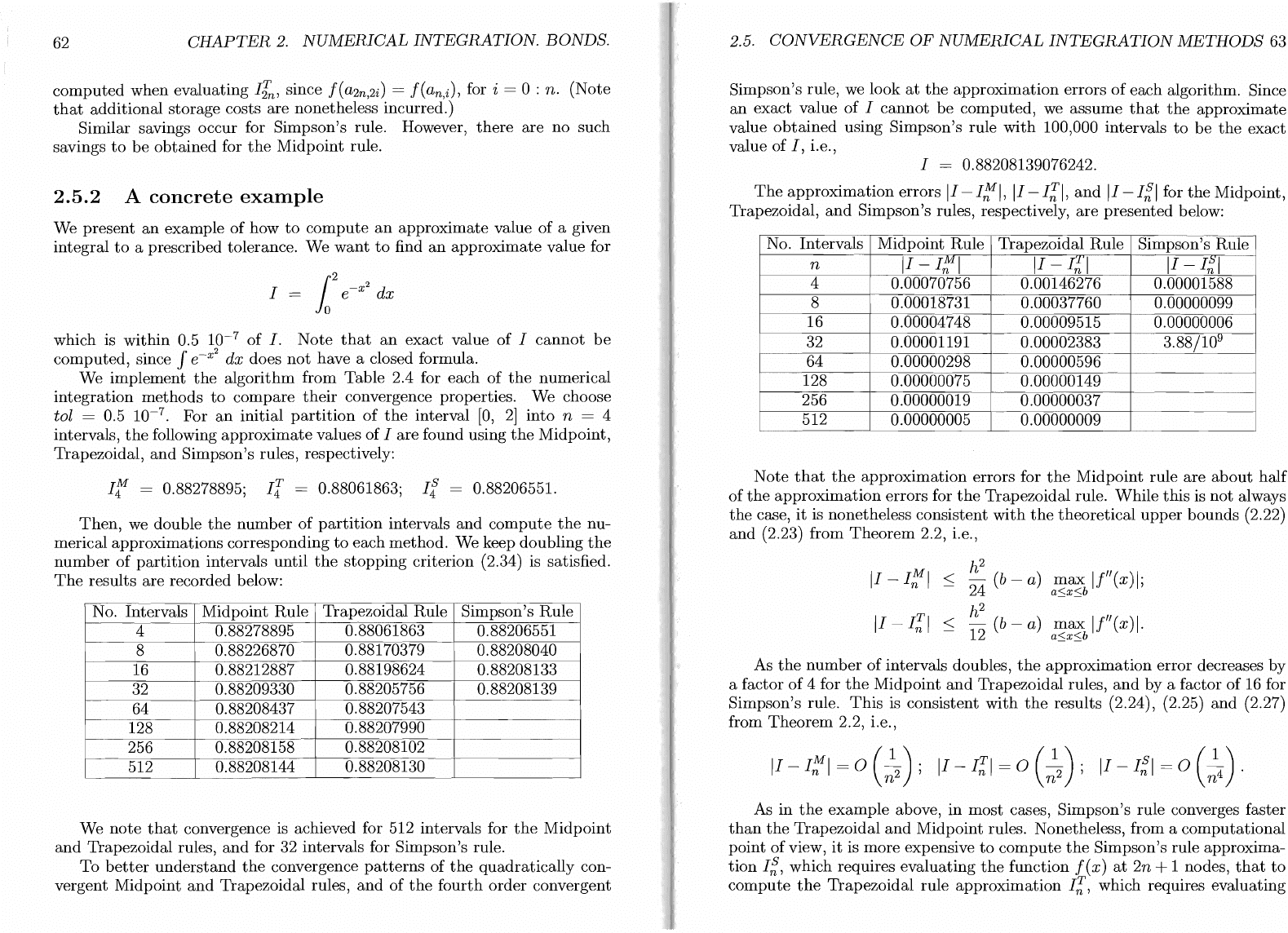
No. Intervals Midpoint
Rule
Trapezoidal Rule Simpson's
Rule
4
0.88278895
0.88061863
0.88206551
8
0.88226870
0.88170379
0.88208040
16
0.88212887
0.88198624
0.88208133
32 0.88209330
0.88205756 0.88208139
64
0.88208437
0.88207543
128
0.88208214
0.88207990
256
0.88208158
0.88208102
512
0.88208144
0.88208130
We
note
that
convergence is achieved for 512 intervals for
the
Midpoint
and
Trapezoidal rules,
and
for 32 intervals for Simpson's rule.
To
better
understand
the
convergence
patterns
of
the
quadratically
con-
vergent Midpoint
and
Trapezoidal rules,
and
of
the
fourth
order
convergent
2.5.
CONVERGENCE
OF
NUMERICAL
INTEGRATION
METHODS
63
Simpson's rule, we look
at
the
approximation
errors
of
each algorithm. Since
an
exact
value
of
I
cannot
be
computed,
we
assume
that
the
approximate
value
obtained
using Simpson's rule
with
100,000 intervals
to
be
the
exact
value of
I,
i.e.,
I = 0.88208139076242.
The
approximation
errors
II
-I~I,
II
-I~I,
and
II
-1%1
for
the
Midpoint,
Trapezoidal,
and
Simpson's rules, respectively,
are
presented
below:
No. Intervals
Midpoint
Rule Trapezoidal
Rule
Simpson's Rule
n
II
-
1%11
II
-
I~
I
II
-
1%1
4
0.00070756 0.00146276
0.00001588
8 0.00018731
0.00037760 0.00000099
16
0.00004748
0.00009515 0.00000006
32
0.00001191
0.00002383
3.88/10
v
64 0.00000298
0.00000596
128
0.00000075 0.00000149
256
0.00000019
0.00000037
512
0.00000005
0.00000009
Note
that
the
approximation
errors for
the
Midpoint
rule are
about
half
of
the
approximation
errors
for
the
Trapezoidal rule.
While
this
is
not
always
the
case,
it
is nonetheless consistent
with
the
theoretical
upper
bounds
(2.22)
and
(2.23) from
Theorem
2.2, i.e.,
II
-
I~I
< h
4
2
(b
-
a)
max
1fl/(x)l;
2
a~x~b
II
I~I
<
h12
(b
-
a)
max
Ifl/(x)l.
2
a~x~b
As
the
number
of
intervals doubles,
the
approximation
error decreases
by
a factor
of
4 for
the
Midpoint
and
Trapezoidal rules,
and
by
a factor
of
16 for
Simpson's rule.
This
is consistent
with
the
results (2.24), (2.25)
and
(2.27)
from
Theorem
2.2, i.e.,
As
in
the
example
above,
in
most
cases,
Simpson's
rule converges faster
than
the
Trapezoidal
and
Midpoint
rules. Nonetheless, from a
computational
point
of
view,
it
is
more
expensive
to
compute
the
Simpson's rule approxima-
tion
1%,
which requires
evaluating
the
function f (x)
at
2n + 1 nodes,
that
to
compute
the
Trapezoidal
rule
approximation
I~,
which requires evaluating