Stacey F.D., Davis P.M. Physics of the Earth

Подождите немного. Документ загружается.

//FS2/CUP/3-PAGINATION/SDE/2-PROOFS/3B2/9780521873628C09.3D

–

127

– [117–134] 13.3.2008 10:36AM

N ¼

2pG

e

zðzÞdz: (9:20)

Equation (9.20) shows that geoid variation is due

to the dipole moment of density above the depth

of compensation, whereas gravity is caused by

the integrated mass. For topography of a given

elevation the depth of the mass contrast deter-

mines the associated geoid anomaly. Deeper

masses give stronger geoid anomalies. Airy iso-

stasy (Fig. 9.6b) is often associated with a crustal

root of low-density material in the mantle, for

example beneath the Himalaya and Andes the

crust extends to depths of 75 km, giving geoid

highs. In regions underlain by hot mantle,

such as mid -ocean ridges and hot spot swells,

as at Hawaii, and regions of continental exten-

sion with thin lithosphere, such as the Basin

and Ran ge of North America, the co mpensa-

tion occurs deeper and the geoid anomalies

are stronger lows.

Measurements of the geoid by what we now

know as astrogeodetic surveying have a history

extending back into antiquity, being the original

method of demonstrating that the Earth is

approximately spherical. It determines the ori-

entation of the vertical, that is the normal to the

geoid, relative to the positions of stars. There was

a rapid development of the method in the early

1700s, when the metre had been defined in

terms of the dimensions of the Earth and parties

of French scientists were sent to various parts of

the world to measure it more precisely. At that

time north–south surveys were much easier than

east–west surveys because they are not critically

dependent on precise timing of the east–west

motions of stars, with the result that the ellip-

ticity of the Earth was well determined. Gravity

surveying developed from this work and espe-

cially from the ideas of M. Bouguer, who was

surveying in South America in the 1730s and

observed deflections of the vertical from a

smooth geoid, caused by extreme topography

in the Andes mountains. He attempted to mea-

sure the Newtonian gravitational constant, G,by

two methods: one by observing the deflection of

the vertical on the slopes of Mount Chimborazo

and the other by comparing gravity on a plateau

and on a low-lying plane, assuming the plateau

to be a superimposed slab with a gravitational

effect given by Eq. (9.19) (Bullen, 1975). He was

thwarted by isostasy and realized that his results

were unsatisfactory, but his work is recognized by

identifying his name with the Bouguer method.

It was an astrogeodetic survey across North India

more than 100 years later that prompted the

recognition of isostasy by J. H. Pratt, who led

the survey party, and G. B. Airy, who, as British

Astronomer Royal, had ultimate responsibility for

the work in India.

The processes of interpreting geoid anoma-

lies by Eq. (9.20) and calculating Bouguer ano-

malies use a flat-earth approximation and are

satisfactory only on scales that are small com-

pared with the radius of the Earth. The anoma-

lies featured in Fig. 9.1 are too extensive for

this approximation to be applied. It is notable

that they are of greater amplitudes than more

local anomalies, which are typically only a few

metres, and this is an indic ation that they h ave a

deep cause. Heterogeneity o f the deep mantle is

implicated and possibly even core–mantle

boundary topography, although it is likely that

the base of the mantle is soft enough for top-

ography to be isostatically balanced with the

heterogeneity in the D

layer at the base of

the mantle.

Particular interest in geoid anomalies arises

from their relationship to dynamics of the man-

tle. Convection is driven by thermally generated

density differences that must be reflected in the

gravity field, but the problem is not a simple one.

The mantle viscosity is strongly dependent on

temperature, as well as being affected by pres-

sure, and the convective pattern has no more

than a remote resemblance to convection in an

isoviscous fluid (Yoshida, 2004). There are also

compositional heterogeneities to confuse the

picture. Nevertheless, some conclusions are

possible. Hager (1984) poin ted out that zones

of strong subduction are correlat ed with geoid

highs, particularly when long-wavelength fea-

tures of the geoid are emphasized by restricting

consideration to low-degree harmonics, whereas

the downwarping, obvious at the trenches,

would be expected to cause lows. His explana-

tion is that the topographic effect is masked by

9.4 GRAVITY AND INTERNAL STRUCTURE 127

//FS2/CUP/3-PAGINATION/SDE/2-PROOFS/3B2/9780521873628C09.3D

–

128

– [117–134] 13.3.2008 10:36AM

resistance to subduction in the deep mantle,

causing a build-up of the dense subducting mate-

rial responsible for the geoid highs and slowing

the subduction, so that the lower-viscosity asthe-

nosphere partially infills the topographic depres-

sions. This requires viscosity to increase with

depth in the mantle by a factor 30 or so, as

most authors claim to be indicated also by post-

glacial rebound (Sections 9.5 and 9.6).

9.5 Post-glacial isostatic

adjustment

Delayed rebound of the Earth from depression

by glacial ice has been recognized for many

years, and Haskell (1935) showed that it can be

applied to a calculation of mantle viscosity. He

obtained a value of 10

Pa s, which is s till used

as a satisfactory global average and is referred to

as ‘the Haskell value’ ( Mitrovica, 1996). More

recent work, directed to the radial variation in

viscosity, is reviewed by Peltier (1982, 2004),

Lambeck (1990), Mitrovica (1996), Mitrovica

and Forte (1997) and Kaufmann and Lambeck

(2000). Information about the depth variation

is conveyed by the geometri cal form of the

rebound and its lateral scale. We illustrate the

principle with two simple models. One is essen-

tially the Haskell model, an isoviscous half

space, but with a superimposed lithosphere,

and the other is a thin asthenosphere, within

which all flow occurs, overlying a rigid mantle

and with a very thin lithosphere that flexes

freely but has no horizontal motion or viscous

flow. The variations in the rate of rebound with

lateral scale are quite different for these models.

While they appear to be extremes, they are both

deficient in not allowing for the flexural

rigidity of the lithosphere. Although the li-

thosphere is defined as the cool and rigid sur-

face layer of the mantle, this definition appeals

to its t emperature-dependent rheology. The

effective thickness for post-glacial rebound is

much less than the thickness apparent from the

study of seismic waves, which stress the litho-

sphere on a time scale that is almost 10

times

shorter. We assess the lithospheric thickness

in Section 20.4 and discuss i ts relevance to

reboundattheendofthissection.

Haskell’s (1935) estimate of mantle viscosity

was based on a record of isostatic rebound of the

glacially depressed area around the Gulf of

Bothnia (Fennoscandia). The heaviest glaciation

and the largest area of rebound are now recog-

nized to be centred on Canada (Laurentia) and are

illustrated by the vertical motions of North

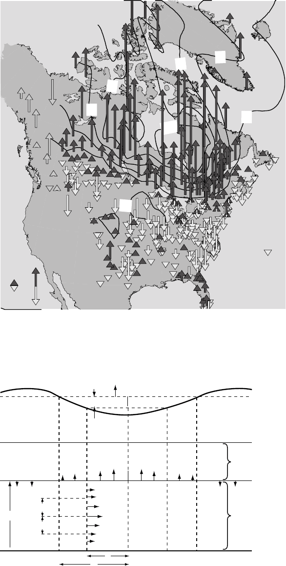
America, as plotted in Fig. 9.7. Peltier (2004)

identified an area to the west of Hudson Bay as

the location of the most rapid current rebound

(1.5 cm/year) and inferred peak ice load (the

Keewatin Dome), but GPS observations of

rebound by Sella et al. (2007) put Hudson Bay itself

at the centre of the action. Haskell (1935) consid-

ered the response of an isoviscous half space to a

circular load with a Gaussian profile of rebound

velocity, and matched his model to the

Fennoscandian data, by a method referred to

below. Availability of data from the larger-scale

Laurentia rebound provides a measure of the

scale dependence of rebound which is important

to inferences about depth dependence of viscos-

ity. Most recent analyses favour an asthenosphere

with viscosity lower by at least an order of magni-

tude and a lower mantle with viscosity up to an

order of magnitude higher than Haskell’s value.

But there are strong lateral variations, so that no

simple radial model can be unambiguous.

We now examine the simple, thin astheno-

sphere model of rebound. Both the upper and

lower boundaries of the asthenosphere behave

as rigid boundaries for the purpose of calculating

the flow. We are modelling the present day flow

and this represents a late stage in the isostatic

adjustment to deglaciation, so we seek a self-

consistent solution in which the local rebound

speed, V

, is everywhere proportional to the

remaining isostatic anomaly in elevation, .

Departures from this state will have been subject

to more rapid adjustment. Thus we can calculate

a rebound time constant, , in terms of the scale

of the flow pattern, where

¼=: (9:21)

The geometry of the flow is represented in

Fig. 9.8. This shows the ‘moat’ of sinking land

128 THE GEOID, ISOSTASY AND REBOUND

//FS2/CUP/3-PAGINATION/SDE/2-PROOFS/3B2/9780521873628C09.3D

–

129

– [117–134] 13.3.2008 10:36AM

–2

IGb00

0–1 5 mm

–1

+ve

–ve

Vertical Velocities

FIGURE 9.7 Laurentia

glacial rebound from GPS

measurements, showing

a region of uplift centred near

Hudson Bay, surrounded by

a moat of subsidence at a

boundary marked by a solid line.

Reproduced, by permission,

from Sella et al. (2007).

Surface Elevation Anomaly

Lithosphere

Asthenospher

FIGURE 9.8 Model of rebound

flow in a sharply bounded

asthenosphere of uniform

viscosity. The radius, R, of a circle

of residual depression is much

larger than the thickness, H, of the

asthenospheric layer in which

flow occurs. The lithosphere

allows vertical movement by

flexure, but does not permit

horizontal flow.

9.5 POST-GLACIAL ISOSTATIC ADJUSTMENT 129

//FS2/CUP/3-PAGINATION/SDE/2-PROOFS/3B2/9780521873628C09.3D

–

130

– [117–134] 13.3.2008 10:36AM

surrounding the uplifting area, as required by

the conservation of material. It is important to

the approximations in this model that the hor-

izontal scale is much larger than the vertical

scale, so that the viscous drag of the horizontal

flow limits the rebound rate. The local driving

forcefortheflowisthedeficiencyinhydro-

static pressure,

P ¼ g; (9:22)

where  ¼3400 kg m

3

is the asthenospheric

density, because it is asthenospheric material

that is displaced, and g ¼9.9 m s

2

is the value

of gravity at that level. The model has circular

symmetry, so that the asthenospheric flow is

radially inwards.

Theflowthroughacentralannulusof

radius r in the asthenosphere is driven by the

pressure gradient, dP/dr. Then the shear stress,

(h), on each of the upper and lower faces of a

central layer of thickness 2h,asinFig.9.8,is

duetothispressuregradientactingoverthe

thickness 2h,

 hðÞ¼

dP=drðÞ2h2pr

2:2pr

h: (9:23)

Therefore the flow speed, v,at(h, r) is given by

¼

 hðÞ



¼g

d



; (9: 24)

where  is the viscosity and Eq. (9.22) gives

the substitution for P. Integrating to level

h from one boundary of t he asthenosphere

at H/2,

v ¼

g



d





; (9:25)

and hence the total volume flow of material

though the annular ring of radius ris

F ¼ 2pr  2

H=2

v dh ¼

gr

d

: (9:26)

The rate of rise of material at radius r is

2pr

g

2r

d

þ r



; (9:27)

so that, by assuming that the form of the resi-

dual depression is preserved, as its amplitude

decreases, and therefore that we can substitute

for V

by Eq. (9.21), we have the differential

equation for (r),



d

12

gH





 ¼ 0: (9:28)

This is the special case (for n ¼0) of Bessel’s

equation



d

þ 1 



 ¼ 0; (9:29)

where

x ¼

12

gH





1=2

r: (9:30)

The solution is therefore the zero-order Bessel

function

 ¼  r ¼ 0ðÞJ

xðÞ: (9:31)

The first zero of this function occurs at x ¼2.4,

so that the radius of the circular depressed area,

R, is given by

12

gH





1=2

R ¼ 2:4: (9:32)

For this model, the time constant for the

approach to isostatic equilibrium is therefore

 ¼ 2:1R

=gH

(9:33)

and, if we make the unknown  the subject of

the equation,

 ¼ 0:48gH

=R

: (9:34)

By this model, the estimated asthenospheric

viscosity depends very strongly on its assumed

130 THE GEOID, ISOSTASY AND REBOUND

//FS2/CUP/3-PAGINATION/SDE/2-PROOFS/3B2/9780521873628C09.3D

–

131

– [117–134] 13.3.2008 10:36AM

thickness, but in reality it is not sharply

bounded.

The other extreme model is an isoviscous

half space, similar to that of Haskell (1935) but

with the addition of a lithosphere that acts as a

frictional boundary and moves only vertically,

not participating in the horizontal flow. Haskell

considered a depression of Gaussian form and,

by Fourier–Bessel analysis, resolved it into a

sum (more correctly, integral) of Bessel func-

tions, each of which retains its form as it decays

and so can be identified with a relaxation time.

The decay of the whole depression is then

obtained from the sum of the individually

decaying Bessel functions, J

, so that it prog res-

sively approaches the form of the most slowly

decaying term. T hus the solution is sup erfi-

cially similar to that of the bounded astheno-

sphere model above, with the most slowly

decaying Bessel term dominating the geometry

at an advanced stage in the recovery. But there

isacrucialdifferencethatwecanseebya

simple dimensional analysis. As in Eq. (9.33),

we require a relaxation time, ,proportionalto

(/g). H does not enter the problem, so the only

other dimensioned quantity involved is the

radius, R, of the depression. Thus, to balance

dimensions we must have

 ¼ C=gR; (9:35)

where C is a dimensionless constant. The two

extreme models lead to very different depend-

ences of t on R, proportionality to R

for the

bounded asthenosphere and 1/R for the uniform

half space.

The areas of Fennoscandian (R 600 km) and

Laurentide (R 1300 km) rebound are suffi-

ciently different that we can use them as a test

of Eqs. (9.34) and (9.35). Since the equations rep-

resent extreme models, and we expect the truth

to lie somewhere between them, we write  / R

with k ¼2 for the thin asthenosphere and k ¼1

for the half space. For Fennoscandia there is good

agreement on the relaxation time, 4600 years

(Mitrovica, 1996) or 4350 years (Peltier, 1998),

but for Laurentia the estimates are seriously

divergent: 6700 years (Mitrovica) or 3400 years

(Peltier). The Mitrovica numbers give k ¼0.49,

midway between the extremes, indicating that,

although the asthenosphere is not sharply

bounded and the deep mantle participates in

the rebound, there is a strong increase in viscos-

ity with depth. The Peltier values give k ¼0.32

and are, therefore, indicative of a much more

nearly isoviscous mantle. Although the models

are greatly simplified, these conclusions coin-

cide with more detailed analyses. Mitrovica

and Forte (1997) and K aufman and Lambeck

(2000) concluded that the increase in viscosity

between the uppermost and lower mantles is of

order a factor 100, whereas Peltier (1998) con-

cluded that the increase at 660 km depth is

no greater than a factor of 5. We need to con-

sider the reason for such different conclusions,

drawn fr om what are essentia lly the same

observations.

As we have mentioned, the simple models

above do not account satisfactorily for the

lithosphere, which imposes a constraint on the

motion in the underlying mantle that depends

on the scale of the motion. This scale depend-

ence is determined by the flexural rigidity of the

lithosphere and is a strong function of its thick-

ness. We discuss the lithospheric thickness in

Section 20.4 and, for flexure on a time scale of

a few thousand years in the continental areas

where rebound is observed, conclude that it is

about 60 km. However, Peltier favoured 120 km

and Lambeck et al. (1996) pointed out that the

thick lithosphere assumed by Peltier accounts

for the relatively slight viscosity contrast across

the mantle in his models and a high estimate of

upper mantle viscosity.

The scale dependence problem draws atten-

tion to the manner in which rebound calculations

are carried out. The current upward surface

motion is identified not with a residual surface

depression but with the history of the ice load

that caused it. The viscosity models rely on ice

history models and are not derived from instanta-

neous measures of relaxation time constants. If

we consider the different spatial harmonic terms

of a rebound pattern (the Fourier–Bessel coeffi-

cients in the Haskell calculation), then they have

different relaxation times, so that the present

pattern depends not only on the history of the

ice load, but on the response to it. Traditionally,

9.5 POST-GLACIAL ISOSTATIC ADJUSTMENT 131

//FS2/CUP/3-PAGINATION/SDE/2-PROOFS/3B2/9780521873628C09.3D

–

132

– [117–134] 13.3.2008 10:36AM

rebound has been observed as the rise of land

relative to sea level, by identification of former

shore lines, now elevated. With allowance for the

rise in sea level itself, this records the history of

the process at specific localities. Now the Grace

satellite presents the opportunity to observe the

present rate of rise globally, and not just at shore

lines. This will provide a resolution of the ques-

tion of the adequacy of the observed rebound to

explain the variation in ellipticity, considered in

the following section.

Viscosity is a controlling parameter in mantle

convection (Chapter 22). In this case the lateral

variations are more significant because subduc-

tion of the cool, almost rigid lithospheric slabs

requires flow in the adjacent mantle. As with

rebound, the flow occurs most readily in

layers of lowest viscosity and a detailed three-

dimensional flow pattern is difficult to model

on a sufficiently fine scale. However, information

about viscosity derived from convection studies

is complementary to that derived from rebound.

The mechanical energy dissipation is thermo-

dynamically related to the heat flux and so

gives a well constrained value of

dV through

the volume of the mantle, where

" is the strain

rate. The model of an almost rigid lithosphere

overlying a weak asthenosphere with strongly

increasing viscosity a greater depths is consis-

tent with the discussion of convective energy in

Section 13.2.

9.6 Rebound and the variation

in ellipticity

Ice-age glaciation was a high latitude phenom-

enon, so that rebound means a slow withdrawal

of mantle material from lower latitudes to infill

the high latitude depressions. A result is a slow

decrease in the gravitational potential coeffi-

cient J

(see Eqs. (6.1), (6.2) and (6.14)) and, as

discussed in Section 6.4, there is a corresponding

effect on the rotation rate, !. First, we consider

the consequence of supposing that the excess J

is a global phenomenon, that is, the Earth as a

whole is flattened. Then J

is related to the sur-

face ellipticity, f ¼(a c)/a, by Eq. (6.20), where

a, c are equatorial and polar radii, and for the

present purpose we can ignore m in this equation

by assuming

¼ð2=3Þ

f . If the surface deforma-

tion is ellipsoidal we can write it as

r ¼J

að3 cos

  1Þ=2; (9:36)

where DJ

is the excess J

attributable to polar

depression. Then the gravitational energy of

the deformation is an integral over the surface

area A,

E ¼ 1=2

gðrÞ

dA ¼ð2p=5Þa

gðJ

; (9:37)

and the energy dissipation by the decreasing J

dE=dt ¼ð4p=5Þa

gð J

: (9:38)

The strain rate is simply

f and so we can write

it as

" ¼

f ¼ð3=2Þ

; (9:39)

and then the dissipation is, in terms of the mean

or effective viscosity,



;

dE=dt ¼

dV ð9=4Þð



ð4p=3Þðr

mantle

 r

core

¼ 7:9a



: ð9:40Þ

Equating (9.38) and (9.40),

 ¼ 0:32 ga½J

¼2:2  10

ðyearsÞ (9:41)

for  in Pa s, because [J

] is the relaxation

time, . If we assume  ¼10

Pa s, the Haskell

value, then  450 years. This just confirms that,

for the isoviscous model, the relaxation time

decreases with scale and that, by this model, a

depression of global extent would now have

recovered to the point of being unobservable.

On the other hand if we apply the simplistic

compromise model,  /R

with k ¼0.5, then the

global scale relaxation time would be about

13 000 years, and if there were ever a significant

global scale depression then it would now be

dominant. Neither of these alternatives appears

plausible, so we consider the consequence of

attributing the J

variation to the sum of the

effects of more local rebound.

132 THE GEOID, ISOSTASY AND REBOUND

//FS2/CUP/3-PAGINATION/SDE/2-PROOFS/3B2/9780521873628C09.3D

–

133

– [117–134] 13.3.2008 10:36AM

SinceLaurentiaisthelargestofthewell-studied

areas of glaciation and rebound, we use it to esti-

mate the ellipticity change that is explained by it.

The effect to be explained is a long-term average

rate of change dJ

=dt 

¼2:8  10

11

year

1

and, if Laurentia accounted for a large part of

this, we could be confident that the process is

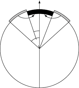
understood. Its rebound is modelled, in the man-

ner of Fig. 9.9, as the development of a uniform

spherical cap of angular radius 

and mass m by

withdrawal of this mass from an annular ring

extending from 

to 

. The moment of inertia of

the cap about its axis (z)is



¼ ma

ð2  cos 

 cos



Þ=3(9:42)

and the moment of inertia of the annular ring

about the same axis is

I

¼ ma

ð3  cos



 cos 

cos 

 cos



Þ=3:

(9:43)

Thus the total change in moment of inertia about

the z axis due to the shift of the mass m is

I

¼I

 I

¼ma

ð1 þ cos 

 cos 

cos 

 cos



Þ=3: ð9:44Þ

We calculate t he changes in moment of iner-

tia about the x and y axes by applying the

rule that for any distribution of mass m on a

spherical surface the sum of the moments of

inertia about three mutually perpendicular

axes is

þ I

¼ 2mR

: (9:45)

(This is seen by writing the moments of inertia

of any mass element Dm at x, y, z about the

three axes as DI

¼Dm(y

þ z

), DI

¼Dm(x

þ z

¼Dm(x

þ y

), so that DI

þDI

¼2Dm

þ y

þ z

) ¼2DmR

, noting that this applies to

all mass elements individually and therefore to

any distribution of mass on a spherical surface.)

In the rebound situation we are considering only

aredistributionofmasswithnochangeinits

total, so that (DI

þDI

) ¼0 and, with sym-

metry about z,

I

¼ I

¼I

=2(9:46)

with DI

given by Eq. (9.44).

We can allow for a misalignment of z with the

rotational axis, c. Let the z axis be at co-latitude y

in the (c–a) plane. Then

I

¼ I

cos

 þ I

sin



¼ I

ðcos

 ð1=2Þsin

Þ;

(9:47)

I

¼ I

sin

 þ I

cos



¼ I

ðsin

 ð1=2Þcos

Þ; (9:48)

I

¼ I

¼ð1=2ÞI

: (9:49)

Here a, b are equatorial axes that are averaged for

the purpose of calculating J

, so that

J

¼½I

ð1=2ÞðI

þ I

Þ=Ma

¼ I

ð9 cos

  3Þ=4Ma

;

(9:50)

where M is the total Earth mass and DI

is given

by Eq. (9.44). Thus, for a rate of mass transfer

into a cap at latitude ,

¼ð

m=MÞð1 þ cos 

 cos 

cos 

 cos



Þð3 cos

  1Þ=4: (9:51)

Using data by Peltier (2004), we estimate

m ¼ 2:1  10

kg=year (of material of astheno-

spheric density 3400 kg m

3

) into a Laurentide

cap of angular radius 

¼158 at co-latitude

 ¼308. The contribution to

depends on what

is assumed for 

. A thin asthenosphere with

rapidly increasing viscosity at greater depth

FIGURE 9.9 The rebound if Laurentia is modelled as

the development of a uniform spherical cap of angular

radius 

and mass m by withdrawal of this mass from

the annular ring extending from 

to 

9.6 REBOUND AND THE VARIATION IN ELLIPTICITY 133

//FS2/CUP/3-PAGINATION/SDE/2-PROOFS/3B2/9780521873628C09.3D

–

134

– [117–134] 13.3.2008 10:36AM

would restrict 

to a band of order 2

¼30 8.

If this value is assumed then the contribution to

is 4.2 10

12

year

1

, 15% of the tota l. An

annular ring twice as wide, that is (



) ¼308,

uld give

; ¼8:6  10

12

year

1

, still only 31%

of the total. If Laurentia is correctly modelled,

then it is not as dominant as supposed. Adding

Fennoscandia would make little di fference,

because not only is the mass flow smaller, but

so is its angular spread. Antarctic rebound is not

as well documented and may be more signifi-

cant than has been recognized, particularly

if the major ice retreat there occurred much

later than in the northern hemisphere, so that

rebound is at an earlier, faster stage. The dis-

crepancy remains to be resolved.

134 THE GEOID, ISOSTASY AND REBOUND

//FS2/CUP/3-PAGINATION/SDE/2-PROOFS/3B2/9780521873628C10.3D

–

135

– [135–148] 13.3.2008 10:35AM

Elastic and inelastic properties

10.1 Preamble

We refer to a material as elastic if it may be

deformed by stress but recovers its original size

and shape when released from the stress. In fact

no material is perfectly elastic, even if subjected

to indefinitely small stresses, but if recovery is

almost complete (say >99%) and, subject only to

inertial delay, effectively instantaneous, a mate-

rial is regarded as elastic. Even for such a mate-

rial we recognize that the slight departure from

perfect elasticity has important consequences,

which include the attenuation of seismic waves.

At high shear stresses departure from ideal ela-

sticity increases sharply. Each material has an

approximate elastic limit or yield point, which

is the magnitude of stress above which inelastic

or permanent deformation starts to become sig-

nificant. This is additional to the recoverable

elastic response and may increase with time at

constant stress. There is no sharp cut-off so that

very prolonged stresses can cause continued very

slow deformation or creep, especially at high

temperatures, as in mantle convection.

Small elastic strains are normally propor-

tional to stress (Hooke’s law). Then the ratio of

stress to strain is an elastic (‘stiffness’) modulus.

Stress is force per unit area, measured in pascals

(Pa  Nm

2

), and strain is a fractional change in

some dimension or dimensions, so that elastic

moduli have the same units as stress, i.e. pascals.

The theory of elasticity, as we normally consider

it, deals only with very small strains, for which

elastic moduli are effectively material constants.

This is infinitesimal strain theory. It describes

elastic deformations in response to stresses that

are very small compared with values of the elas-

tic moduli. Pressure in the deep interior of the

Earth is much too large for this assumption to

be even approximately valid. In this situation

an elastic modulus must be defined as the ratio

of a small change in stress to the consequent

small strain increment, superimposed on a

much larger ambient compression. The moduli

all increase systematically with pressure and a

more general, finite strain theory is required.

This is a subject of Chapter 18.

Elasticity theory is simplest for materials that

are isotropic, that is having properties that are

the same in all directions. They include polycrys-

talline materials with randomly oriented crys-

tals, such as undeformed metals or igneous

rocks, as well as glassy or amorphous substances.

Elastically isotropic materials have two inde-

pendent elastic moduli. There are several ways

of choosing these moduli, depending on the

form of the strain to be represented, but since

only two can be independent it follows that any

one of them can be represented in terms of any

other two, as summarized in Appendix D. In

seismology and much other geophysics we gen-

erally prefer to use bulk modulus, K, and rigidity

modulus, , as the two independent moduli. The

particular reason for geophysical interest in bulk

modulus is that it provides a link between seis-

mologically observed elastic wave speeds and

the density profile of the Earth. With a minor

proviso concerning the elasticity of a composite

(Section 10.4), the combination of P-wave speed,

//FS2/CUP/3-PAGINATION/SDE/2-PROOFS/3B2/9780521873628C10.3D

–

136

– [135–148] 13.3.2008 10:35AM

controlled by the modulus  (Eq. (10.5)), and

shear wave speed, controlled by rigidity, , pro-

vides a direct observation of the ratio K/ ¼dP/d,

where  is density and P is pressure.

A pure shear strain with no change in volume,

described by , involves no change in temper-

ature and  is unambiguous. On the other hand,

a pure compression with no change in shape,

which is described by K, requires specification

of the conditions under which the compression

is applied. If temperature is maintained constant

we have the isothermal modulus, K

, but if the

material is thermally isolated or if the compres-

sion is too rapid to allow any transfer of heat, as

in a seismic P wave, then the temperature rises

and a higher, adiabatic modulus, K

, applies. This

allows for the fact that compression is partially

offset by thermal expansion. The two principal

bulk moduli, K

and K

, are related by an identity

¼ K

ð1 þ TÞ (10:1)

(T is temperature,  is volume expansion co-

efficient and g is the dimensionless Gr ¨uneisen

parameter, which has numerical values between

1.0 and 1.5 in the Earth). In the deep Earth

the difference between K

and K

is between 4%

and 10%. The other moduli, considered in the

following section, all describe deformations

involving changes in both volume and shape,

so that relationships between isothermal and

adiabatic versions are inconveniently compli-

cated. Equation (10.1) is one of the thermody-

namic identities that link bulk modulus to

other properties, such as thermal expansion

(Appendix E). Rigidity (and therefore also the

other moduli that can be regarded as combina-

tions of K and , as in Appendix D) are not subject

to comparable controls. This means that, when

we consider effects such as the temperature

dependences of moduli (Section 17.5), rigidity

cannot be treated with the same thermodynamic

rigour as bulk modulus and further assumptions

are needed.

For many purposes isotropy is an adequate

approximation, but elastic anisotropy is well rec-

ognized in both the mantle and the solid inner

core. It can arise both from an alignment of

crystals, which are individually anisotropic, and

from the layering of materials with different

properties. The simplest crystals are those with

cubic structures, which have three independent

moduli, but more general anisotropies, requir-

ing a larger number of moduli, are normal in

minerals. The most general situation of a crystal

completely lacking structural symmetry is rep-

resented by 21 moduli (for a reason outlined in

Section 10.3). Although mineralogists face such

complications, in the Earth the form of aniso-

tropy most commonly considered in detail is

uniaxial, that is, having properties in one dir-

ection differing from those in the perpendicular

plane, within which there is no variation. In the

upper mantle the single axis is assumed to be

vertical (radial) and seismologists refer to such a

structure as transversely isotropic. It is repre-

sented by five moduli (Section 10.3). Although

azimuthal anisotropy occurs, both on continents

(e.g. Davis, 2003) and on the ocean floors, on a

global scale gravity selects the vertical axis as

unique. Transverse anisotropy is smeared out

statistically, so that transverse isotropy is to be

expected as a global average. In the inner core it

appears that the rotational axis is selected as a

unique direction. This is best explained by the

precipitation of added material predominantly

on its equator and deformation towards the equi-

librium ellipticity (Yoshida et al., 1996).

Our understanding of the Earth’s interior is

derived almost entirely from seismology and its

interpretation, based on elastic and inelastic

properties. These properties include anisotropy,

the behaviour of composites and polycrystalline

materials, effects of temperature and pressure

and the frequency variation of elasticity, all of

which need to be understood to make maximum

use of seismological data.

10.2 Elastic moduli of an

isotropic solid

The simplest derivation of the relationships

between moduli starts with Young’s modulus,

E, and Poisson’s ratio, , which are defined with

the other moduli in Table 10.1. Consider a rec-

tangular prism, as in Fig. 10.1, with axes x, y, z,

chosen to be parallel to the principal stresses, 

136 ELASTIC AND INELASTIC PROPERTIES