Shiffman Daniel. Learning processing
Подождите немного. Документ загружается.


272 Learning Processing
int xloc = x + i-offset;
int yloc = y + j-offset;
int loc = xloc + img.width*yloc;
// Make sure we haven't walked off the edge of the pixel array
loc = constrain(loc,0,img.pixels.length-1);
// Calculate the convolution
rtotal += (red(img.pixels[loc]) * matrix[i][j]);
gtotal += (green(img.pixels[loc]) * matrix[i][j]);
btotal += (blue(img.pixels[loc]) * matrix[i][j]);
}
}
// Make sure RGB is within range
rtotal = constrain(rtotal,0,255);
gtotal = constrain(gtotal,0,255);
btotal = constrain(btotal,0,255);
// Return the resulting color
return color(rtotal,gtotal,btotal);
}
}
Exercise 15-10: Try diff erent values for the convolution matrix.
Exercise 15-11: Using the framework established by our image processing examples, create
a fi lter that takes two images as input and generates one output image. In other words, each
pixel displayed should be a function of the color values from two pixels, one from one image
and one from another. For example, can you write the code to blend two images together
(without using tint( ) )?
15.10 Creative Visualization
You may be thinking: “ Gosh, this is all very interesting, but seriously, when I want to blur an image or
change its brightness, do I really need to write code? I mean, can’t I use Photoshop? ” Indeed, what we have
achieved here is merely an introductory understanding of what highly skilled programmers at Adobe do. e
power of Processing, however, is the potential for real-time, interactive graphics applications. ere is no need
for us to live within the confi nes of “ pixel point ” and “ pixel group ” processing.
Following are two examples of algorithms for drawing Processing shapes. Instead of coloring the shapes
randomly or with hard-coded values as we have in the past, we select colors from the pixels of a PImage
object. e image itself is never displayed; rather, it serves as a database of information that we can exploit
for our own creative pursuits.
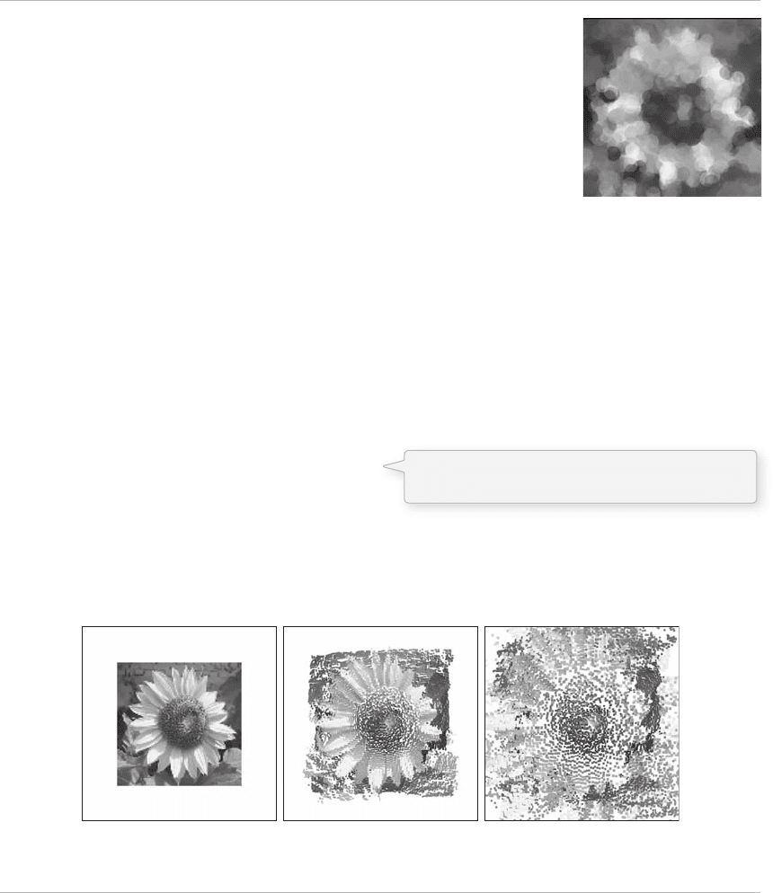
In this fi rst example, for every cycle through draw( ) , we fi ll one ellipse at a random location onscreen
with a color taken from its corresponding location in the source image. e result is a “ pointillist-like ”
eff ect. See Figure 15.16 .
It is often good when looking at
neighboring pixels to make sure
we have not gone off the edge
of the pixel array by accident.
We sum all the neighboring pixels multiplied by
the values in the convolution matrix.
After the sums are constrained within a range of
0–255, a new color is made and returned.
Images 273
Example 15-14: “ Pointillism ”
PImage img;
int pointillize = 16;
void setup() {
size(200,200);
img = loadImage( "sunflower.jpg");
background(0);
smooth();
}
void draw() {
// Pick a random point
int x = int(random(img.width));
int y = int(random(img.height));
int loc = x + y*img.width;
// Look up the RGB color in the source image
loadPixels();
float r = red(img.pixels[loc]);
float g = green(img.pixels[loc]);
float b = blue(img.pixels[loc]);
noStroke();
// Draw an ellipse at that location with that color
fill(r,g,b,100);
ellipse(x,y,pointillize,pointillize);
}
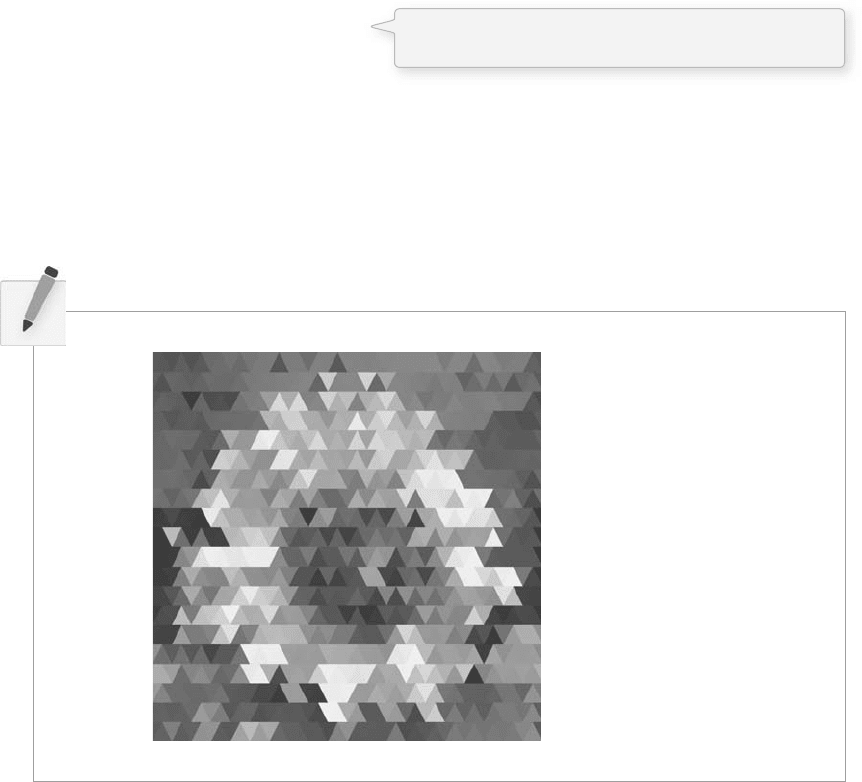
In this next example, we take the data from a two-dimensional image and, using the 3D translation
techniques described in Chapter 14, render a rectangle for each pixel in three-dimensional space. e
z location is determined by the brightness of the color. Brighter colors appear closer to the viewer and
darker ones further away.
fi g. 15.17
fi g. 15.16
Example 15-15: 2D image mapped to 3D
PImage img; // The source image
int cellsize = 2; // Dimensions of each cell in the grid
int cols, rows; // Number of columns and rows in our system
void setup() {
size(200,200,P3D);
Back to shapes! Instead of setting a pixel, we
use the color from a pixel to draw a circle.
274 Learning Processing
img = loadImage( " sunflower.jpg " ); // Load the image
cols = width/cellsize; // Calculate # of columns
rows = height/cellsize; // Calculate # of rows
}
void draw() {
background(0);
loadPixels();
// Begin loop for columns
for (int i = 0; i < cols; i + + ) {
// Begin loop for rows
for (int j = 0; j < rows; j + + ) {
int x = i*cellsize + cellsize/2; // x position
int y = j*cellsize + cellsize/2; // y position
int loc = x + y*width; // Pixel array location
color c = img.pixels[loc]; // Grab the color
// Calculate a z position as a function of mouseX and pixel brightness
float z = (mouseX/(float)width) * brightness(img.pixels[loc])- 100.0;
// Translate to the location, set fill and stroke, and draw the rect
pushMatrix();
translate(x,y,z);
fill(c);
noStroke();
rectMode(CENTER);
rect(0,0,cellsize,cellsize);
popMatrix();
}
}
}
Exercise 15-12: Create a sketch that uses shapes to display a pattern that covers an entire
window. Load an image and color the shapes according to the pixels of that image.
e following image, for example, uses triangles.
A z value for 3D translation is calculated as a function
of the pixel’s brightness as well as mouse location.
Video 275
16 Video
“ I have no memory. It’s like looking in a mirror and seeing nothing but mirror. ”
—Alfred Hitchcock
In this chapter:
– Displaying live video.
– Displaying recorded video.
– Creating a software mirror.
– How to use a video camera as a sensor.
16.1 Before Processing
Now that we have explored static images in Processing , we are ready to move on to moving images,
specifi cally from a live camera (and later, from a recorded movie). Using a digital video camera connected
to a PC or Mac requires a few simple steps before any code can be written.
On a Mac:
• Attach a camera to your computer.
• Make sure any necessary software and drivers for the camera are installed.
• Test the camera in another program, such as iChat, to make sure it is working.
On a PC:
• Attach a camera to your computer.
• Make sure any necessary software and drivers for the camera are installed.
• Test the camera. (Use whatever software that came with your camera that allows you to view the
video stream.)
• Install QuickTime (version 7 or higher). If you are using a previous version of QuickTime, you must
make sure you choose “ custom ” installation and select “ QuickTime for Java. ”
• You will also need to install a vdig (video digitizer) that allows QuickTime applications (what we
are creating) to capture video in Windows. The vdig situation is in flux so I recommend you check
this book’s web site for updates. Although no longer being developed, a free vdig is available at
this site: http://eden.net.nz/7/20071008/ . You can also consider using Abstract Plane’s vdig
( http://www.abstractplane.com.au/products/vdig.jsp ), which costs a small fee, but has more advanced
features.
Admittedly, the process is a bit less complicated on a Mac. is is because Processing uses the
QuickTime libraries in Java to handle video. On Apple computers, QuickTime comes preinstalled
(although sometimes software updates can cause issues), whereas on Windows, we have to make sure we
have taken the steps to install and properly confi gure QuickTime. At the end of this chapter, we will see

276 Learning Processing
that there are few third party libraries available in Processing that do not require QuickTime for video
capture on Windows.
Exercise 16-1: Hook a camera up to your computer. Does it work in another program (not
Processing)? If you are on a PC, install a vdig and test.
16.2 Live Video 101
Once you have made sure you have a working camera connected to your machine, you can start
writing Processing code to capture and display the image. We begin by walking through the basic
steps of importing the video library and using the Capture class to display live video.
Step 1. Import the Processing video library.
If you skipped Chapter 12 on Processing libraries, you might want to go back and review the details.
ere is not much to it here, however, since the video library comes with the Processing application.
All you need to do is import the library. is is done by selecting the menu option Sketch → Import
Library → video, or by typing the following line of code (which should go at the very top of your
sketch):
import processing.video.*;
Using the “ Import Library ” menu option does nothing other than automatically insert that line into your
code, so manual typing is entirely equivalent.
Step 2. Declare a Capture object
We learned in Chapter 12 how to create objects from classes built into the Processing language. For
example, we made PImage objects from the Processing PImage class. PImage, it should be noted, is part of
the processing.core library and, therefore, no import statement was required. e processing.video library has
two useful classes inside of it—Capture, for live video, and Movie, for recorded video. We will start with
declaring a Capture object.
Capture video;
Step 3. Initialize the Capture object.
e Capture object “ video ” is just like any other object. As we learned in Chapter 8, to construct an object,
we use the new operator followed by the constructor. With a Capture object, this code typically appears
in setup( ) , assuming you want to start capturing video when the sketch begins.
video = new Capture();
Video 277
e above line of code is missing the appropriate arguments for the constructor. Remember, this is not
a class we wrote ourselves so there is no way for us to know what is required between the parentheses
without consulting the reference. e online reference for the Capture constructor can be found on the
Processing web site at:
http://www.processing.org/reference/libraries/video/Capture.html
e reference will show there are several ways to call the constructor (see overloading in Chapter 23 about
multiple constructors). A typical way to call the Capture constructor is with four arguments:
void setup() {
video = new Capture(this,320,240,30);
}
Let’s walk through the arguments used in the Capture constructor.
• this —If you are confused by what this means, you are not alone. We have never seen a reference
to this in any of the examples in this book so far. Technically speaking, this refers to the instance
of a class in which the word this appears. Unfortunately, such a definition is likely to induce head
spinning. A nicer way to think of it is as a self-referential statement. After all, what if you needed to
refer to your Processing program within your own code? You might try to say “ me ” or “ I. ” Well, these
words are not available in Java, so instead we say “ this. ” The reason we pass “ this ” into the Capture
object is we are telling it: “ Hey listen, I want to do video capture and when the camera has a new
image I want you to alert this applet. ”
• 320 —Fortunately for us, the first argument, this , is the only confusing one. 320 refers to the width of
the video captured by the camera.
• 240 —The height of the video.
• 30 —The desired framerate captured, in frames per second (fps). What framerate you choose
really depends on what you are doing. If you only intend to capture an image from the camera
every so often when the user clicks the mouse, for example, you would not need a high framerate
and could bring that number down. However, if you want to display full motion video onscreen,
then 30 is a good bet. This, of course, is simply your desired framerate. If your computer is too
slow or you request a very high resolution image from the camera, the result might be a slower
framerate.
Step 4. Read the image from the camera.
ere are two strategies for reading frames from the camera. We will briefl y look at both and somewhat
arbitrarily choose one for the remainder of the examples in this chapter. Both strategies, however, operate
under the same fundamental principle: we only want to read an image from the camera when a new frame is
available to be read .
In order to check if an image is available, we use the function available( ) , which returns true or false
depending on whether something is there. If it is there, the function read( ) is called and the frame from
the camera is read into memory. We do this over and over again in the draw( ) loop, always checking to
see if a new image is free for us to read.
278 Learning Processing
void draw() {
if (video.available()) {
video.read();
}
}
e second strategy, the “ event ” approach, requires a function that executes any time a certain event,
in this case a camera event, occurs. If you recall from Chapter 3, the function mousePressed( ) is
executed whenever the mouse is pressed. With video, we have the option to implement the function
captureEvent( ) , which is invoked any time a capture event occurs, that is, a new frame is available from
the camera. ese event functions ( mousePressed( ), keyPressed( ), captureEvent( ) , etc.) are sometimes
referred to as a “ callback. ” And as a brief aside, if you are following closely, this is where this fi ts in. e
Capture object, “ video, ” knows to notify this applet by invoking captureEvent( ) because we passed it a
reference to ourselves when creating “ video. ”
captureEvent( ) is a function and therefore needs to live in its own block, outside of setup( ) and draw( ) .
void captureEvent(Capture video) {
video.read();
}
To summarize, we want to call the function read( ) whenever there is something for us to read and we can
do so by either checking manually using available( ) within draw( ) or allowing a callback to handle it
for us— captureEvent( ) . Many other libraries that we will explore in later chapters (such as network and
serial) will work exactly the same way.
Step 5. Display the video image.
is is, without a doubt, the easiest part. We can think of a Capture object as a PImage that changes over
time and, in fact, a Capture object can be utilized in an identical manner as a PImage object.
image(video,0,0);
All of this is put together in Example 16-1 .
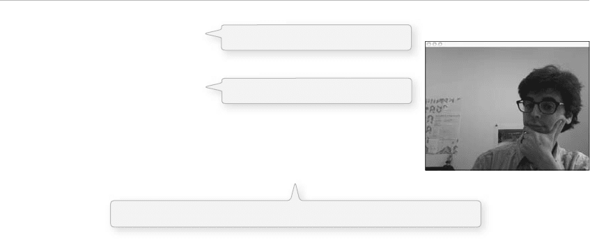
Example 16-1: Display video
// Step 1. Import the video library
import processing.video.*;
// Step 2. Declare a Capture object
Capture video;
void setup() {
size(320,240);
// Step 3. Initialize Capture object via Constructor
// video is 320 x 240, @15 fps
video = new Capture(this,320,240,15);
}
fi g. 16.1
Step 1. Import the video library!
Step 2. Declare a Capture object!
Step 3. Initialize Capture object! This starts the capturing process.

Video 279
void draw() {
// Check to see if a new frame is available
if (video.available()) {
// If so, read it.
video.read();
}
// Display the video image
image(video,0,0);
}
Again, anything we can do with a PImage (resize, tint, move, etc.) we can do with a Capture object.
As long as we read( ) from that object, the video image will update as we manipulate it. See
Example 16-2 .
Example 16-2: Manipulate video image
// Step 1. Import the video library
import processing.video.*;
Capture video;
void setup() {
size(320,240);
video = new Capture(this,320,240,15);
}
void draw() {
if (video.available()) {
video.read();
}
// Tinting using mouse location
tint(mouseX,mouseY,255);
// Width and height according to mouse
image(video,0,0,mouseX,mouseY);
}
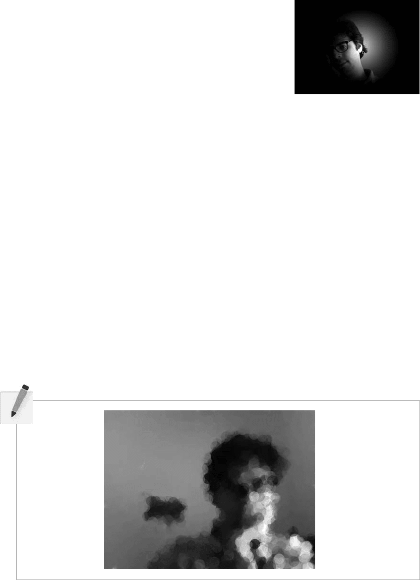
Every single image example from Chapter 15 can be recreated with video. Following is the “ adjusting
brightness ” example (15-19) with a video image .
Example 16-3: Adjust video brightness
// Step 1. Import the video library
import processing.video.*;
// Step 2. Declare a Capture object
Capture video;
void setup() {
size(320,240);
// Step 3. Initialize Capture object via Constructor
video = new Capture(this,320,240,15); // video is 320 x 240, @15 fps
background(0);
}
fi g. 16.2
Step 4. Read the image from the camera.
Step 5. Display the image.
A video image can also be tinted
and resized just as with a PImage.
280 Learning Processing
void draw() {
// Check to see if a new frame is available
if (video.available()) {
// If so, read it.
video.read();
}
loadPixels();
video.loadPixels();
for (int x = 0; x video.width; x + + ){
for (int y = 0; y video.height; y + + ) {
// calculate the 1D location from a 2D grid
int loc = x + y*video.width;
// get the R,G,B values from image
float r,g,b;
r = red (video.pixels[loc]);
g = green (video.pixels[loc]);
b = blue (video.pixels[loc]);
// calculate an amount to change brightness based on proximity to the mouse
float maxdist = 100;// dist(0,0,width,height);
float d = dist(x,y,mouseX,mouseY);
float adjustbrightness = (maxdist-d)/maxdist;
r * = adjustbrightness;
g * = adjustbrightness;
b * = adjustbrightness;
// constrain RGB to make sure they are within 0-255 color range
r = constrain(r,0,255);
g = constrain(g,0,255);
b = constrain(b,0,255);
// make a new color and set pixel in the window
color c = color(r,g,b);
pixels[loc] = c;
}
}
updatePixels();
}
fi g. 16.3
Exercise 16-2: Recreate Example 15-14 (pointillism) to work with live video.
Video 281
16.3 Recorded Video
Displaying recorded video follows much of the same structure as live video. Processing ’s video library
only accepts movies in QuickTime format. If your video fi le is a diff erent format, you will either have to
convert it or investigate using a third party library. Note that playing a recorded movie on Windows does
not require a vdig.
Step 1. Instead of a Capture object, declare a Movie object.
Movie movie;
Step 2. Initialize Movie object.
movie = new Movie(this, "testmovie.mov");
e only necessary arguments are this and the movie’s fi lename enclosed in quotes. e movie fi le should
be stored in the sketch’s data directory.
Step 3. Start movie playing.
Here, there are two options, play( ) , which plays the movie once, or loop( ) , which loops it continuously.
movie.loop();
Step 4. Read frame from movie.
Again, this is identical to capture. We can either check to see if a new frame is available, or use a callback
function.
void draw() {
if (movie.available()) {
movie.read();
}
}
Or:
void movieEvent(Movie movie) {
movie.read();
}
Step 5. Display the movie.
image(movie,0,0);
Example 16-4 shows the program all put together.
