Sarma D.D. Geostatistics with Applications in Earth Sciences
Подождите немного. Документ загружается.


56 Geostatistics with Applications in Earth Sciences
Fig. 3.7 Observed and fitted distributions to the
logarithms
of
gold grade values.
Accumulation
Table 3.6 Fitting
of
lognormal distribution to copper accumu lation values
Class interval Mid Pt. Observed Expected
(O, - E
i
)2
(cm%) frequency
(0)
frequ ency (E)
E
i
I- 50
25.50 9
11
.45 0.524
50- 150
100.00 30 31.99 0.123
150
-250
200.00 27 24.50 0.255
250
-350
300.00 14 9.01 2.760
350--450 400.00
5
4.94
450
-550
500.00 5
3.27
550-650 600.00
I 2.28
650
-750
700.00
I 13
1.65
14.05
0.078
750
-850
800.00 0
1.23
850
-950
900.00 0 0.95
950- 1050 1000.00 I 0.74
Total 94 93.60 3.740
Since the computed Chi-square value (3.740) is less than the theoretical
Chi-square value (5.991) at 5% level
of
significance and (5 - 2 - 1) = 2
degrees
of
freedom , we infer that the fitting
of
log normal distrib ution to the
copper accumulation values is justified.
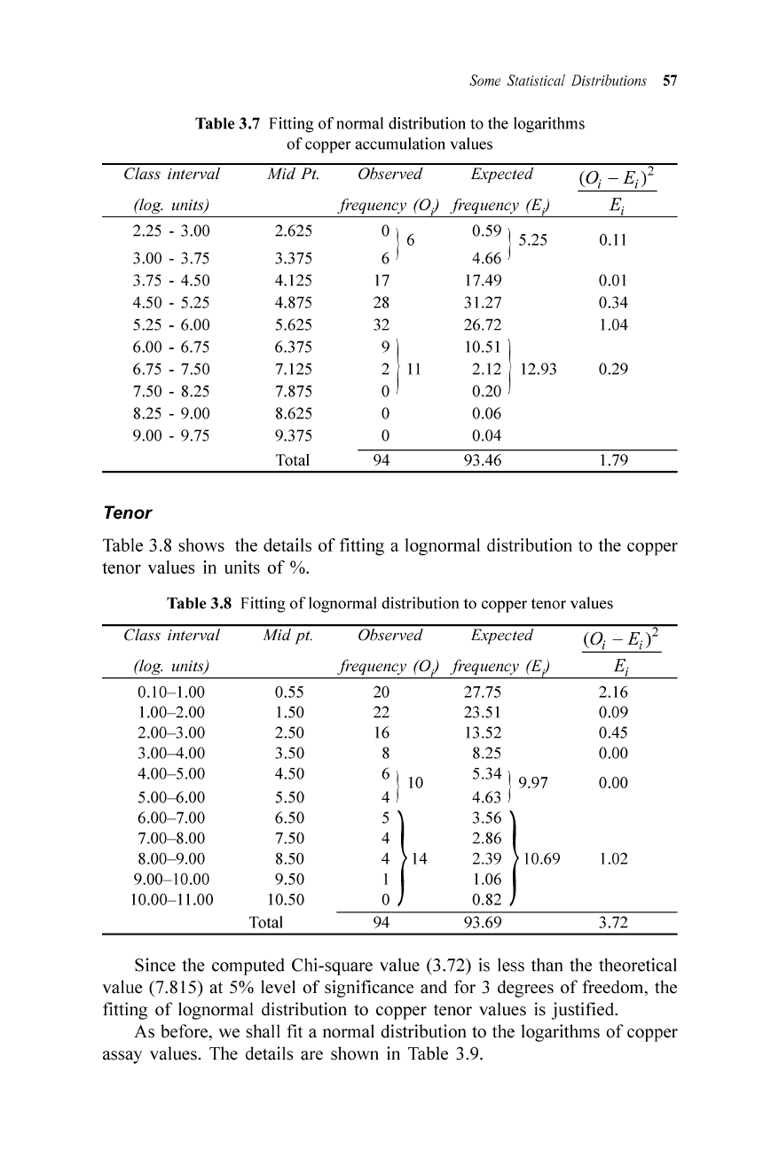
As before we shall show the details
of
fitting a normal distr ibution to
the logarithms
of
copper accumulation values. The details are shown in
Table 3.7.
Since the computed Chi-square value (1.79) is less than the theoretical
Chi-square value (5.99 1) at 5% level
of
significance and (5 - 2 - 1) = 2
degrees
of
freedom , we infer that the fitting
of
normal distrib ution to the
logarithms
of
copper accumulation values is justified.
Som
e Statistical Dis
tribu
tion
s 57
Table 3.7 Fitting of normal distribution to the logarithms
of copper accumulation values
Class interval Mid Pt. Observed Expected
(log. units)
fr
equency
(0)
fr
equency
(E)
2.25 - 3.00 2.625
~
) 6
0.59
)5
.25
3.00 - 3.75 3.375
4.66
3.75 - 4.50
4.125 17 17.49
4.50 - 5.25 4.875 28 31.27
5.25 - 6.00 5.625 32 26.72
6.00 - 6.75 6.375 9 10.51
6.75 - 7.50 7.125 2
11
2.12 12.93
7.50 - 8.25 7.875 0 0.20
8.25 - 9.00 8.625 0 0.06
9.00 - 9.75 9.375 0 0.04
Total 94 93.46
Tenor
0.11
0.01
0.34
1.04
0.29
1.79
Table 3.8 shows the details
of
fitting a lognormal distribution to the
copper
t
enor
values in units
of
%.
Table 3.8 Fitting
of
lognormal distribution to copper tenor values
Class interval Mid pt. Observed Expected
(O, - E
i
)2
(log. units)
fr
equency
(0)
f requency (
E)
t:
0.10-1.00
0.55
20 27.75 2.16
1.00
-2
.00
1.50 22 23.51 0.09
2.00
-3
.00
2.50 16 13.52 0.45
3.00--4.00
3.50 8
8.25
0.00
4.00
-5
.00 4.50
~
) 10
5.34
)9
.97
0.00
5.00
-6
.00 5.50
4.63
6.00
-7
.00
6.50
}4
3
56
}
7.00
-8
.00
7.50
2.86
8.00- 9.00
8.50
2.39 10.69 1.02
9.00- 10.00
9.50 1.06
10.00-11 .00 10.50 0.82
Total 94 93.69 3.72
Since the computed Chi- square value (3.72) is less than the theoretic al
value (7.815) at 5% level
of
significance and for 3
degr
ees
of
freedom, the
fitting
of
lognormal distribution to
copper
tenor values is
ju
stified.
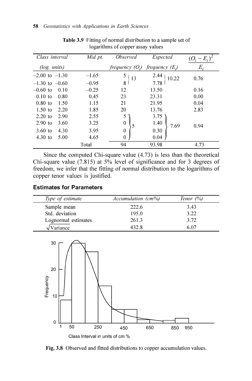
As before, we shall fit a normal distribution to the logarithms
of
copper
assay values. The detail s are shown in Table 3.9.
58
Geostatistics with Applications in Earth Sciences
Table 3.9 Fitting
of
normal distribution to a samp le set
of
logarithms
of
copper assay values
Class interval Mid pt. Observed Expected
2
(OJ - E
j
)
(log. units) frequency
(0)
frequency
(E)
E
j
- 2.00 to - 1.30 - 1.65
~
)13
2.44 ) 10.22
0.76
- 1.30 to
-0.60
- 0.95
7.78
- 0.60 to 0.10 - 0.25 12 13.50 0.16
0.10 to 0.80 0.45 23 23.31 0.00
0.80 to 1.50 1.15 21 21.95 0.04
1.50 to 2.20 1.85 20 13.76 2.83
2.20 to 2.90 2.55
D5
375
)
2.90 to
3.60
3.25
1.40 7.69
0.94
3.60 to
4.30
3.95 0.30
4.30 to
5.00
4.65 0.04
Total 94 93.98 4.73
Since the computed Chi-square value (4.73) is less than the theoretical
Chi-square value (7.8 15) at 5% level
of
significance and for 3 degrees
of
freedom, we infer that the fitting
of
normal distribution to the logarithms
of
copper tenor values is justified.
Estimates for Parameters
Type
of
estimate
Sample mean
Std. deviation
Lognormal estimates
.JVariance
30
20
()'
c:
Q)
::J
xr
~
u..
10
Accumulation (cm%)
222.6
195.0
261.3
432.8
Tenor (%)
3.43
3.22
3.72
6.07
50
250
450
650
850 950
Class Interval in units of em %
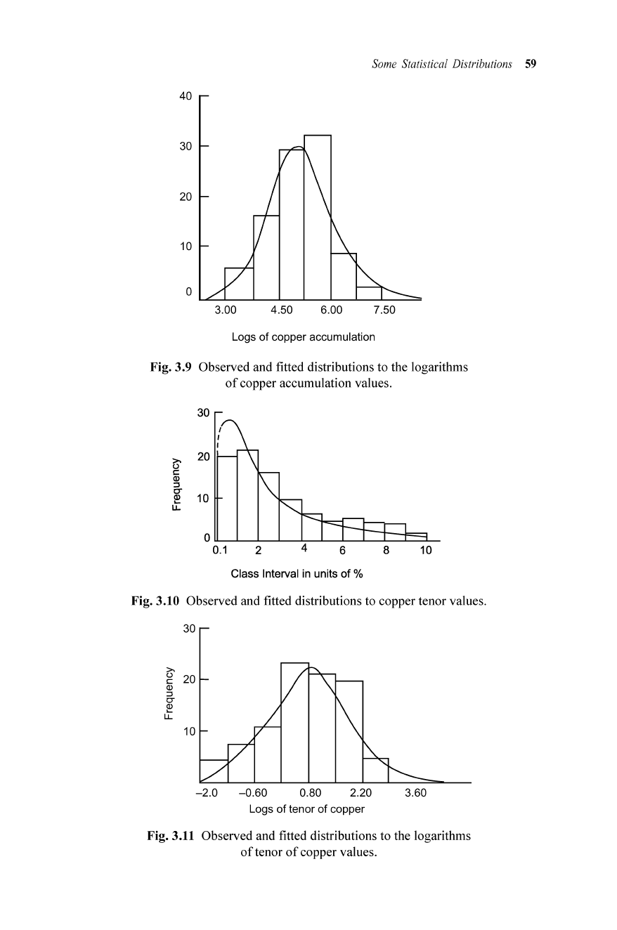
Fig. 3.8 Observed and fitted distributions to copper accumu lation values.
Some Statistical Distributions 59
40
30
20
10
o
'--"'--'---'---'--'----'--'---'---=
3.00 4.50 6.00 7.50
Logs of copper accumulation
Fig.3.9
Observed and fitted distributions to the logarithms
of
copper accumulat ion values.
30
10
Class Interval in units of %
10
Fig.3.10 Observed and fitted distributions to copper tenor values.
30
~
c 20
Q)
::::>
0-
~
lJ..
10
-2.0
-0.60
0.80 2.20 3.60
Logs of tenor of copper
Fig.3.11 Observed and fitted distributions to the logarithms
of
tenor
of
copper values .

60 Geostatistics with Applications in Earth Sciences
3.5
CASE OF REJECTION OF NORMAL DISTRIBUTION
So far we have discussed the cases
of
fitting normal distrib utions to Fe
20
3
values, and also fitting normal and lognormal distributions in the following
cases.
S.No. Deposit Variable Fitted distribution
I.
Gold ore Accumulation (cm-gms) Lognormal
2. Gold ore
Accumulation (cm-gms)
Normal to logarithms
accumulation
3.
Gold ore Grade (gms /tonne) Lognormal
4. Gold ore Grade (gms/tonne) Normal to logarithms
of
grade
5.
Copper Accumulation (cm-%) Lognormal
6. Copper
Accumulation (cm-%)
Normal to logarithms
of
accumulation
7. Copper
Tenor (%)
Lognormal
8. Copper
Tenor (%)
Normal to logarithms
of
tenor
For a change, let us first fit normal distribution to copper tenor values
and see what would result from the application
of
Chi-square test. The
copper assay values which are 94 in number were listed in Chapter 2.
The observed distrib ution and the fitted normal distrib ution to these data
together with the application
of
Chi-square test are shown in Table 3. 10.
Tab
le 3. 10 Fitting
of
normal distribution to a set
of
copper assay values
Class interval Mid point Observed Expected
fr
equency
fr
equency
0.00 - 1.00
0.5
20 06.12
1.00 - 2.00
1.5
22 11.50
2.00 - 3.00
2.5 16 16.72
3.00 - 4.00 3.5 08
17.10
4.00 - 5.00 4.5
06
16.31
5.00 - 6.00
5.5 05
10.02
6.00 - 7.00
6.5 05 07.50
7.00 - 8.00
7.5
04
03.50
8.00 - 9.00 8.5 03 02.39
9.00 - 10.0
9.5 01 00.99
10.0 - 11.0
10.5 00 12 00.81 8.57
11.00- 12.0 11.5 01 00.52
12.00-13.0 12.5
00
00.23
13.00-14.0 13.5 02
00.09
13.00-15.0
14.5 00 00.03
15.00-16.0
15.5 00 00.01
16.00-17.0
16.5 0 1 00.00
Total 94 93.64
31.48
9.58
0.00
5.08
6.52
2.52
0.83
1.37
57.38
Some Statistical Dis
tribu
tions
61
1210
'Observed
25
20
>-
15
o
c:
Q)
:>
CT
10
~
LL.
5
0
0
2 4 6 8
Class Interval
(%)
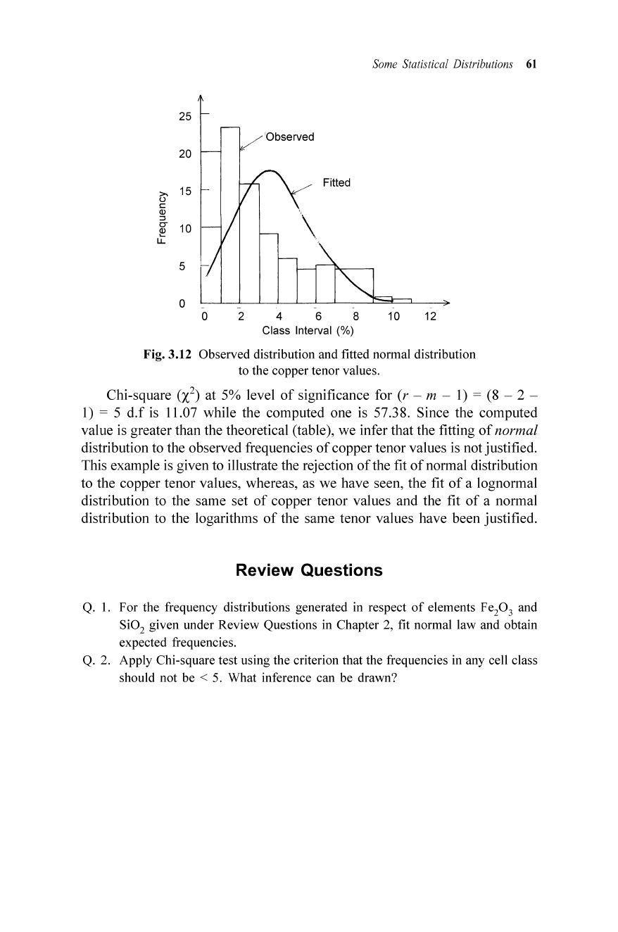
Fig.3.12 Observed distribution and fitted normal distribution
to the copper tenor values .
Chi-square (X
2
) at 5% level
of
significance for (r - m - I) = (8 - 2 -
1) = 5
d.f
is 11.07 while the computed one is 57.38. Since the computed
value is greater than the theoretical (table), we infer that the fitting
of
normal
distribution to the observed frequencies
of
copper tenor values is not justified.
This example is given to illustrate the rejection
of
the fit
of
normal distribution
to the copper tenor values, whereas, as we have seen, the fit
of
a lognormal
distribution to the same set
of
copper tenor values and the fit
of
a normal
distribution to the logarithms
of
the same tenor values have been justified.
Review Questions
Q. I. For the frequency distributions generated in respect
of
elements Fep 3 and
Si0
2
given under Review Questions in Chapter 2, fit normal law and obtain
expected frequencies.
Q. 2. Apply Chi-square test using the criterion that the frequencies in any cell class
should not be < 5. What inference can be drawn?
4
Stochastic
Modelling (Time
Series
Analysis)
and
Forecasting
4.1 INTRODUCTION
One
of
the objectives
of
statistical analysis
of
sequences
of
data is to draw
inferences about the properties
of
the population from which these sequences
of
samples are drawn . Prediction
of
future observations is done by construct-
ing relevant models based on stochastic process concepts. Stochastic processes
can be classified as stationary and non-stationary. Special classes
of
linear
models
of
stationary stochastic processes are:
I. Auto-regressive processes (AR),
2. Moving-average (MA) and
3. Auto-regressive and moving average processes (ARMA).
4.1.1 Stochastic Processes
Stochastic process may be described as a phenomenon unfolding in 'time'
according to certain probability laws. Here, the word 'time' is used as a real
variable which may not always stand for time. When such inference is
subjected to certain laws
of
probability, it can be described in terms
of
random
variables 21' 2
2
,
2
3
, . . .
2
11
,
each 2 corresponding to one instant
of
time. As
the number
of
time units or instants increase abundantly, we are obliged to
consider the situation
of
a multivariate. The assemblage
of
these random
variables together with their probability distributions is called as Stochastic
Process. A geological process may be viewed as a stochastic process because
it is associated with different geochemical elements
-each
of
which can be
treated as Random Variable having a probability distribution. Here the
observations are not in time, but in space. Even then, we can apply the time-
domain models
of
stochastic processes (time series analysis) to geological
processes. The applicability
of
a stochastic process and in particular, the
subclasses, viz. AR, MA and ARMA , depends on the behaviour
of
the
relevant autocorrelation function (act) and the partial autocorrelation function
(pact). An excellent treatment
of
these models may be seen in Box and
Jenkins (1976) .

S
tocha
stic Modelling
(Tim
e Series Analysis) and Forecasting 63
4.1.2 The Autocorrelation Function (acf)
For a sequence
of
observations
zl'
z2'
...
, zn' the autocorrelation coefficient
at lag
'k' is defined as: P
k
= E[(zi-
Il)(z
i+k-
Il
)]/
~E(Z
i
-1l)2
E(zi+k
-1l)2
, where
E stands for the expectation or expected value. For a stationary process, the
variance is the same at time
t + k as at t. For k = 0,
Po
= 1. The plot
of
autocorrelation coefficients PI' P2' ... Pkas a function
of
lag (k) is called the
autocorrelation function
of
the process. Generally speaking,
if
the
'acf
' is
of
(i) infinite damped exponentials and/damped sine waves form , the process
is autoregressive; (ii)
ifit
cuts the X-axi s (finite), it is mov ing average (MA),
and (iii)
if
it is infinite damped exponentials and/or damped sine wav es after
q-p first lags, then the process is autoregressive and moving average model
(ARMA).
Standard Error
of
Autocorrelation Estimates
In the process
of
identification
of
the appropriate model, it is nece ssary to
verify in the first instance, whether the population autocorrelation coefficient
P
k is zero beyond a certain lag k. Bartlett (1946) has given an approximate
expression for the variance
of
the estimated autocorrelation coefficient (r
k
)
of
a stationary Normal process and this can be used for the said purpose.
+
~
Var(r
k
)
==
~
I
{p~
+Pv
+
kP
v-
k
-4P
kP
vPv-
k
+2p~p
l}
(4.1)
V = -cx::>
The variance
of
the estimated autocorrelations r
k
at lags k > some value
q beyond which the theoretical autocorrelation function may be treated as
petered out. Bartlett's approximation gives:
q
Var (rk)
==
~
{I + 2 I
p~},
k > q
v =1
Standard Error (S.E) =
~Var(r
k)
.
(4.2)
If the assumption is that the series is completely random, we have q =
0. Therefore, for all lags, r
k
is zero and hence Var (r
k)
:::
~
.
S.E = .JVar .
Employing these statistics,
95%
confidence limits (± 1.96 S.E) can be worked
out for the autocorrelations. Any points exceeding these limits can be
considered as significant.
Partial Autocorrelation Function (pact)
The quantity
<P
kk regarded as a function
of
the lag k is called the partial auto-
correlation function (see eqn. 4.5 below).
The partial autocorrelation coefficients may be estimated by fitting suc-
cessively autoregressive proce sses
of
order I, 2, 3 ... by least squares and
, , ,
picking up the estimates
<P1I'
<P22
'
<P3
3' ...
of
the last coefficient fitted at each
64 Geostatistics with Applications in Earth Sciences
stage. There are,
of
course, other methods
of
estimation;
(i)
if
the 'pa
cf
' is
finite or cuts-off, the process is autoregressive, (ii)
if
it is infinite i.e. domi-
nated by damped exponentials and/or sine waves, the process is moving
average and (iii)
if
it is infinite i.e., dominated by damped exponentials and!
or sine waves after first p-q lags or tails-off, it is auto-regressive and moving
average (integrated) model. For more details , please see Box and Jenkins
(1976) . Thus, depending on the information provided by
acf
and
pacf
, we
decide on the class
of
models to be chosen , viz., AR, MA, or ARMA.
Standard Error
of
Partial Autocorrelation Estimates
Quenouille (1949) has shown that on the hypothesis that the process is
autoregressive
of
order p , the estimated partial autocorrelations
of
order
p + I and higher are approximately independently distributed with variance
==
~
for k
~
p + I. The standard error (S.E)
of
the estimated partial auto-
correlation
<1>kk
is
S.E
(<1>
kk) =
~
for k
~
p + 1
Employing this, 95% confidence limits can be worked out for the partial
autocorrelation coefficients. Any points exceeding these limits can be con-
sidered as significant.
4.2 STOCHASTIC MODELLING (TIME SERIES ANALYSIS)
A linear random process may be described by a linear filter model
of
the
type:
(4.3)
where 2t = Zt -
11,
'¥
l'
'¥
2' .
..
are filter coefficients and
11
= mean
of
the
process. The sequence
at
(usually referred to by communication engineers as
white noise series) has zero mean and variance
cr~.
The
11
is a parameter that
describes the level
of
the process zr If the process is stationary,
11
is the mean
of
Zt process. We may also assume that
11
has been estimated
(z)
and
removed from the time-series. Thus 2t = Zt - z. The process 2t will, there-
fore, describe a zero mean process . The model defined by equation (4.3)
implies that 2t can be written alternatively as a weighted set
of
past values
of
a t' plus an added shock noise/error i.e.,
or simply,
2
t
= 1t
1
2
t
_
1
+ 1t
2
2
t
_
2
+ ... + a t
and a finite version may be written as:
2
t
=
<1>pl
2
t
_
1
+
<1>p
2
2
t
-2
+ ... +
<1>pp2
t
_
p
+
at
2
t
=
<1>1
2
H
+
<1>2
2
t-2 + ... +
<1>p2
t_p
+ a t
(4.4)
(4.5)
S
tocha
stic Modelling
(Tim
e Series Analysis) and Forecasting 65
The model represented by (4.5) is known as autoregressive model
of
order p i.e., AR(P). It may be seen that this is a regression model and Z is
said to be regressed on
the
previous values itself; hence
the
name
'autoregressive'. The autoregressive model is a special case
of
the linear
filter model represented by (4.3). For example we estimate ZI- I from the
RHS
of
(4.5) by substituting
2
1
-
1
=
<1>1
2
1-
2
+
<1>2
2
1
-
2
+
<1>
3
2
1-
3
+ ... + a
l
_
1
(4.6)
Similarly, we substitute for 2
1
-
2
and so on. Ultimately we arrive at
infinite series in the a's.
From (4.5), we write,
AR(I)
as:
2
1
=
<1>1
2t-! + a
l
(4.7)
4.2.1 Physical
Significance
in Relation
to
Estimation
of
Blocks
of
Ore
Consider the set-up given in Fig. 4.1.
~-3
~-1
Fig
.4
.1 An example
of
auto-regressive set-up
of
a sequence
of
blocks
of
ore.
We are interested in estimating the average grade
of
the block, ZI (shaded
area), given the previous grades
of
the blocks ZI_ 1' z l_2'
...
,
zl
_k' Let us suppose
that the block values are detrended by subtracting the mean value z from
each. If AR(1) model is chosen , it means that the block ZI is estimated by
giving proper weightage to the immediately preceding block z
l_I
' Suppose,
the average grade z is 4.0 gms and the block 2
1
-
1
has a grade
of
6 gms/
tonne
of
ore and the weight coefficient
<1>1
(AR coefficient) is 0.8. Then, the
estimated value for ZI is 0.8 x 6.0 = 4.8 + 4.0 = 8.8 gms/tonne
of
ore. Let
us extend the logic to AR(2) model. We write 2
1
=
<1>1
2I- I +
<1>2
2
1-2
+ a t' In
order to estimate ZI' we need the grades
of
the immediately preceding two
blocks. If the grades
of
2
1
- 1' 2
1
-
2
blocks are say 8 gms and 6 gms respectively
and the weight coefficients are 0.6 and 0.5 respectively, the estimated grade
for ZI is 8.0 x 0.6 + 6.0 x 0.5 + 4.0 = 11.8 gms/tonne
of
ore. If the order
is p , in order to estimate ZI' we consider the immediately preceding p blocks
of
z t' Every estimate has an error associated with it. Following Box and
Jenkin s (1976), for
AR(I)
model, the variance function at lead time 'L' for
AR( 1) model is:
(4.8)
