Sarma D.D. Geostatistics with Applications in Earth Sciences
Подождите немного. Документ загружается.


2
Univariate Statistical Methods,
Frequency
Analysis
and
Simulation
2.1 UNIVARIATE STATISTICAL METHODS
We may recall that from the statistical point
of
view, the totality
of
possible
experimental outcomes may be called 'population'
of
the outcomes, while a
set
of
data obtained by performing the experiment a number
of
times is
called 'sample' from the population. Since it is time consuming, uneconomical
and may not be practical to analyse the whole population, statistical inference
consists in drawing conclusions on the basis
of
its samples drawn. The type
of
information extracted from a set
of
data depends upon its input and the
model selected.
Geological populations can be sampled and numerical expressions
obtained. For example, the tenor
of
copper in a mineral deposit or the grade
of
ore in a gold deposit or the elements' concentration in bauxite deposits
(AI
20
3
,
Fe
20
3
etc.) at various sampling points or the number
of
zircon grains
in a microscope slide etc., can be obtained for statistical analysis. If we are
considering one variable, it becomes univariate as against multivariate
corresponding to multivariables. When two variables are considered, the
specific term is bivariate.
2.2 FREQUENCY ANALYSIS
Usually, an earth scientist faces the problem
of
comprehending a huge number
of
observations. These observations could be realisations
of
a random variable,
say grade
of
ore. To draw inferences, one must order these observations by
grouping and averaging. For this purpose, we resort to frequency analysis.
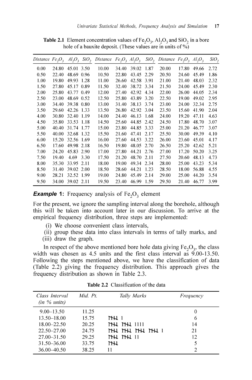
In Table 2.1, a sample set
of
sixty Fe
20
3
,
Al
20
3
and
Si0
2
element
concentration values in units
of
% are given.
Univariate Statistical Methods, Frequency Analysis and Simulation 17
Table 2.1 Elementconcentration values of Fe
20
3
,
AI
20
3
and
Si0
2
in a bore
hole of a bauxite deposit. (These values are in units of %)
Distance Fe
lO
3
AIP 3 Si
al
Distance
F
ep
3 AIP 3
Si
al
Distance Fe
l
O
3
AIP 3
S
ia
l
0.00 24.80 45.01 3.50 10.00 34.40 39.02 1.87 20.00 17.80 49.66 2.72
0.50
22.40 48.69 0.96 10.50 22.80 43.45 2.29 20.50 24.60 45.49
1.86
1.00
19.80 49.93 1.28 11.00 26.60 42.58 3.91 2 1.00 21.40 48.03 2.32
1.50
27.80 45.17 0.89 11.50 32.40
38.72
3.34 21.50 24.00 45.49 2.30
2.00 25.80 43.77 0.49 12.00 27.40 42.92 4.34 22.00 26.00 44.05 2.34
2.50 23.00 48.69 0.52 12.50 25.80 43.89 3.20 22.50 19.00 49.02 2.95
3.00
34.40
39.38 0.80
13.00 31.40 38.13 3.74 23.00 24.00 32.34 2.75
3.50 29.60 42.26 1.33 13.50 26.80 42.92 3.04 23.50 15.60 41.90 2.04
4.00 30.80 32.40 1.19 14.00 24.40 46.13 1.68 24.00 19.20 47.11 4.63
4.50 35.80 33.53 1.18 14.50 25.60 44.85 2.42 24.50 17.80 48.70 3.07
5.00 40.40 3 1.74 1.77 15.00 23.80 44.85 3.33 25.00 21.20 46.77 3.07
5.50 40.00 32.68 1.32 15.50 21.60 47.41 2.17 25.50 30.00 49.39 4.10
6.00 15.20 32.56 1.69 16.00 27.60 44.53 3.22 26.00 23.60 45.01 4.17
6.50
17.60 49.98 2.18 16.50 19.80 48.05 2.70 26.50 25.20 42.62 5.21
7.00
24.20 45.83 2.90 17.00 27.80 44.21 2.76 27.00 17.20 50.20 3.25
7.50
19.40 4.69
3.30
17.50 21.20 48.70 2.11
27.50
20.60 48.13 4.73
8.00 35.30
33.95 2.11 18.00 19.00 49.34 2.34 28.00 25.00 43.23 5.34
8.50
31.40 39.02 2.00 18.50 28.60 44.21 1.23 28.50 18.00
56.88
4.55
9.00
28.21 32.52 1.99 19.00 24.80 45.49 2.14 29.00 25.00 44.20 3.54
9.50
34.00 39.02 2.11 19.50 23.40 46.99
1.59
29.50 21.40 46.77
3.99
Example 1: Frequency analysis
of
Fe
2
0
3
element
For the present , we ignore the sampling interval along the borehole, although
this will be taken into account later in our discussion. To arrive at the
empirical frequency distribution, three steps are implemented:
(i) We choose convenient class interv als,
(ii) group these data into class intervals in terms
of
tally marks, and
(iii) draw the graph.
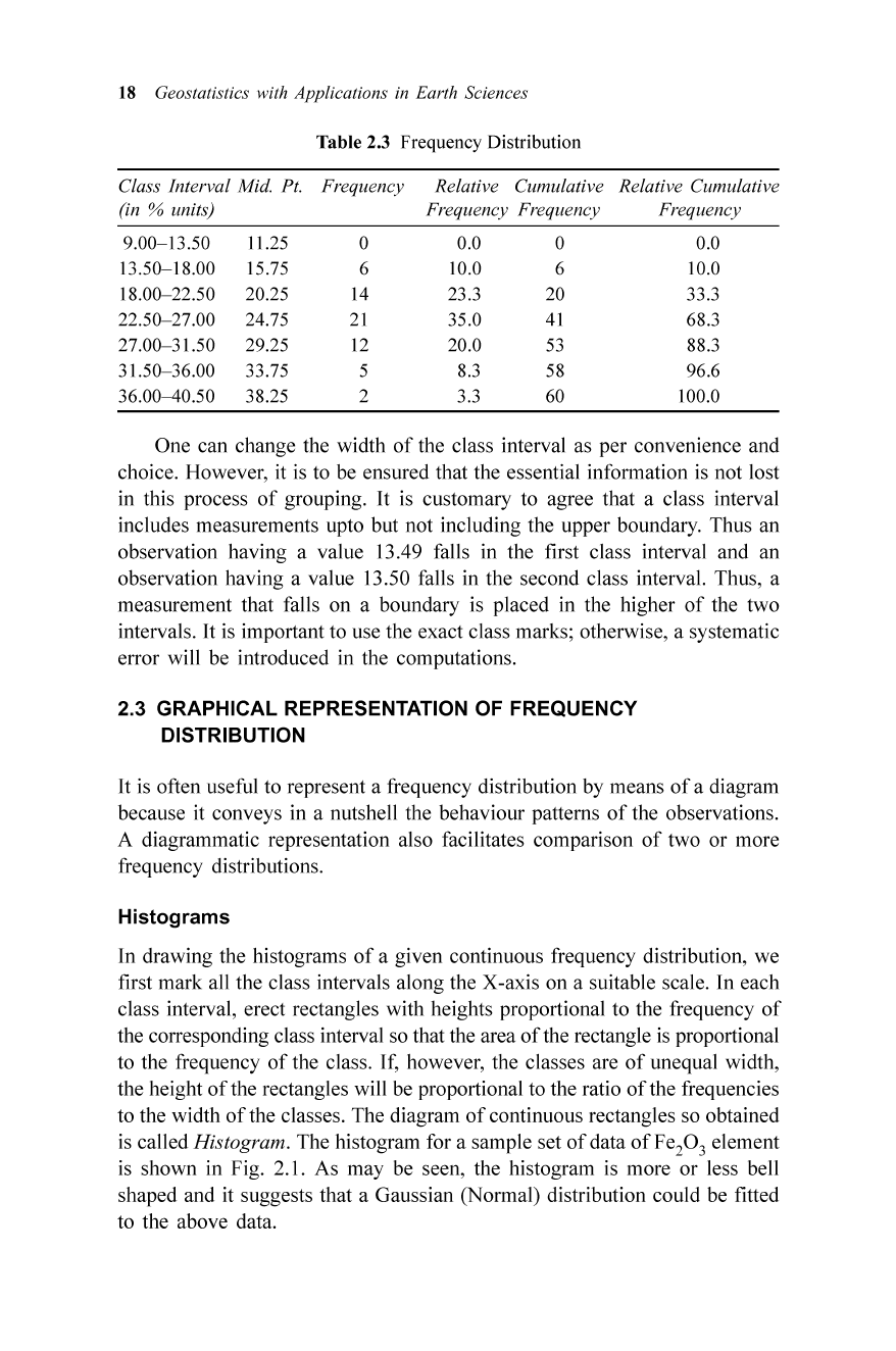
In respect
of
the above mentioned bore hole data giving Fe
2
0
3
,
the class
width was chosen as
4.5 units and the first class interval as 9.00-13 .50.
Following the steps mentioned above, we have the classification
of
data
(Table 2.2)
giving
the frequency distribution. This approach
give
s the
frequency distribution as shown in Table 2.3.
Table 2.2 Classification of the data
Class Int
erva
l
Mid
. Pt. T
all
y
Marks
Fr
equ
ency
(in
% units)
9.00
-13
.50 11.25
0
13
.50
-18
.00 15.75
fH.l
1
6
18
.00
-22
.50
20 .25
fH.l
fH.l
1111 14
22
.50
-27
.00
24 .75
fH.l
fH.l
fH.l
fH.l
1 21
27
.00
-31.50
29 .25
fH.l fH.l
11 12
31
.50
-36
.00
33 .75
fH.l
5
36
.00-40
.50 38 .25 11 2
18 Geostatistics with Applications in Earth Sciences
Ta ble 2.3 Frequency Distribution
Class Interval Mid. Pt. Frequency Relative Cumulative Relative Cumulative
(in
% units) Frequency Frequency Frequency
9.00- 13.50
11.25 0 0.0 0 0.0
13.50
-18
.00
15.75 6 10.0 6 10.0
18.00
-22
.50 20.25 14 23.3 20
33.3
22.50
-27
.00 24.75 21
35.0
41
68.3
27.00
-31
.50 29.25 12 20.0
53 88.3
31.50
-36
.00
33.75 5 8.3 58 96.6
36.00--40.50 38.25 2
3.3 60
100.0
One can change the width
of
the class interval as per convenience and
choice. However, it is to be ensured that the essential information is not lost
in this process
of
grouping. It is customary to agree that a class interval
includes measurements upto but not including the upper boundary. Thus an
observation having a value 13.49 falls in the first class interval and an
observation having a value 13.50 falls in the second class interval. Thus, a
measurement that falls on a boundary is placed in the higher
of
the two
intervals. It is important to use the exact class marks; otherwise, a systematic
error will be introd uced in the computations.
2.3 GRAPHICAL REPRESENTATION OF FREQUENCY
DISTRIBUTION
It is often useful to represent a freque ncy distribution by means
of
a diagram
because it conveys in a nutshell the behaviour patterns
of
the observations.
A diagrammatic representation also facilitates comparison
of
two or more
frequency distributions.
Histograms
In drawing the histograms
of
a given continuous frequency distribution, we
first mark all the class intervals along the X-axis on a suitable scale. In each
class interval, erect rectangles with heights proportional to the frequency
of
the corresponding class interval so that the area
of
the rectangle is proportional
to the frequency
of
the class. If, however, the classes are
of
unequal width,
the height
of
the rectang les will be proportional to the ratio
of
the frequencies
to the widt h
of
the classes. The diagram
of
continuous rectangles so obtained
is called
Histogram.
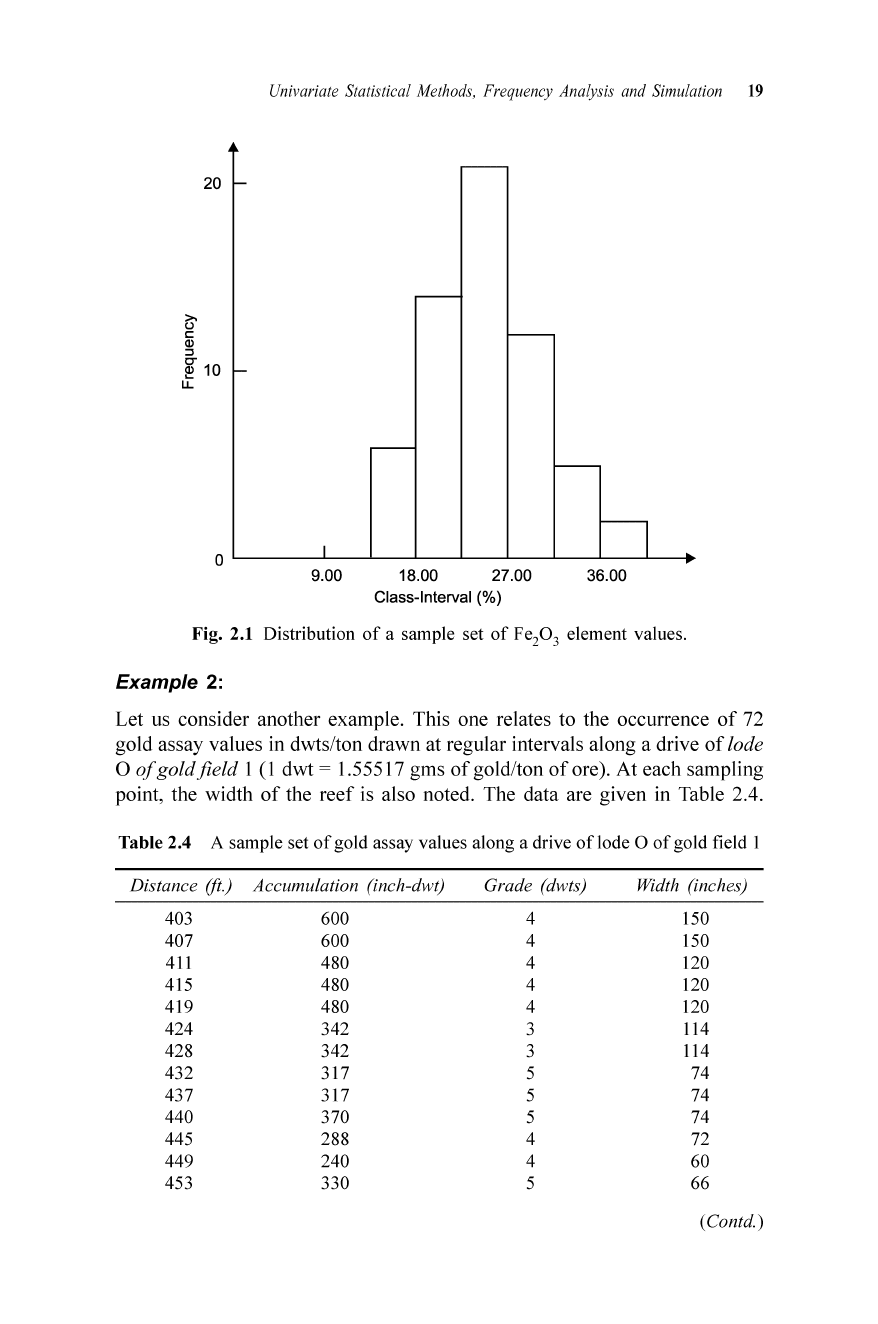
The histogram for a sample set
of
data
of
Fe
2
0
3
element
is shown in Fig.
2. 1. As may be seen, the histogram is more or less bell
shaped and it suggests that a Gaussian (Normal) distrib ution could be fitted
to the above data .
Univ
ariate Statistical Methods, Frequency Analysis and
Simu
lation
19
20
I-
~
c
OJ
::l
~
10
l-
LL
n
36.00
Fig. 2.1 Distribution
of
a sample set
of
Fe
20
3
element values.
Example 2:
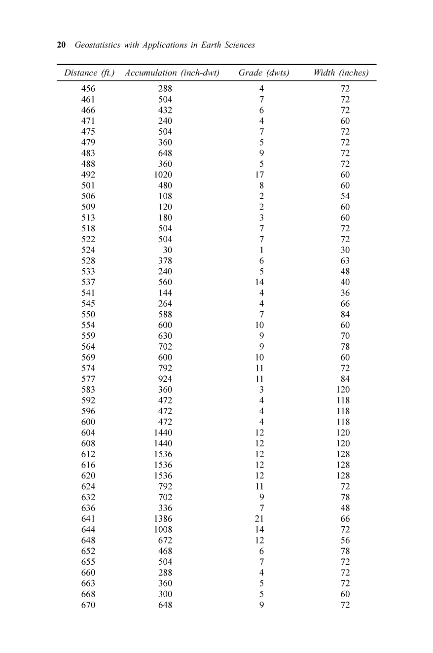
Let us consider another example. This one relates to the occurrence
of
72
gold assay values in dwts/ton drawn at regular intervals along a drive
of
lode
o
of
gold
fi
eld I (I dwt = 1.55517 gms
of
gold/ton
of
ore). At each sampling
point, the width
of
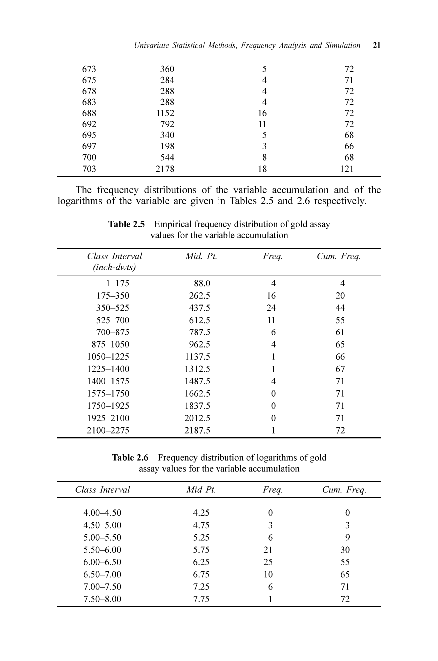
the reef is also noted. The data are given in Table 2.4.
Table
2.4 A sample set
of
gold assay valu es along a driv e
of
l
ode
°
of
gold field I
Distance (ft.) Accumulation (inch-dwt)
403 600
407 600
411
480
415 480
419 480
424 342
428 342
432 317
437 317
440 370
445 288
449 240
453 330
Grade (dwts)
4
4
4
4
4
3
3
5
5
5
4
4
5
Width (inches)
150
150
120
120
120
114
114
74
74
74
72
60
66
(Contd.)
20 Geostatistics with Applications in Earth Sciences
Distance
(ft.) Accumulation (inch-dwt) Grade (dwts) Width (inches)
456 288 4 72
461 504
7 72
466 432 6 72
471
240 4
60
475 504
7 72
479 360 5 72
483 648
9 72
488 360 5 72
492
1020
17
60
501 480 8 60
506 108 2 54
509
120
2
60
513 180 3 60
518 504
7 72
522 504 7 72
524
30
I
30
528
378 6 63
533 240 5 48
537 560 14 40
541
144
4
36
545 264 4 66
550 588 7
84
554
600
10
60
559 630 9 70
564 702
9 78
569 600 10 60
574
792
11
72
577 924
11
84
583 360 3 120
592 472 4
118
596 472 4
11
8
600 472 4
11
8
604
1440
12 120
608 1440 12 120
612
1536
12 128
616
1536
12
128
620 1536 12 128
624
792
11
72
632 702 9 78
636 336 7
48
641
1386
21 66
644
1008
14
72
648 672 12 56
652 468
6 78
655 504 7 72
660
288 4
72
663 360 5 72
668 300 5 60
670 648 9 72
Univariate Statistical Methods, Frequency Analysis and Simulation 21
673
675
678
683
688
692
695
697
700
703
360
284
288
288
11
52
792
340
198
544
2178
5
4
4
4
16
11
5
3
8
18
72
71
72
72
72
72
68
66
68
121
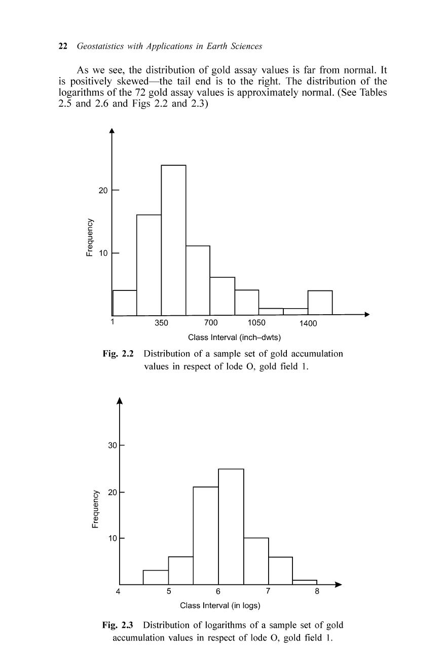
The frequency distributions
of
the variable accumulation and
of
the
logarithms
of
the variable are given in Tables 2.5 and 2.6 respectively.
Table 2.5 Empirical frequency distribution
of
gold assay
values for the variable accumu lation
Class Int
erval
Mid. Pt. Freq. Cum. Freq.
(inch-dwts)
1-175 88.0 4 4
175
-350
262.5 16 20
350-525
437.5 24 44
525-700 612.5
II
55
700-875
787.5
6 61
875-1050
962.5 4
65
1050
-1225
1137
.5 I
66
1225
-1400
1312
.5 I 67
1400
-1575
1487
.5 4
71
1575
-1750
1662
.5
0
71
1750
-1925 1837.5
0
71
1925
-2100 2012.5
0
71
2100-2275 2187.5 I
72
Tab le 2.6 Frequency distribution
of
logarithms
of
gold
assay values for the variable accumu lation
Class Inter val
Mid
Pt. Freq. Cum. Freq.
4
.00--4
.50 4.25
0 0
4.50-5 .00
4.75
3 3
5.00-5 .50
5.25
6 9
5.50
-6
.00 5.75
21
30
6.00
-6
.50 6.25 25 55
6.50
-7
.00 6.75
10
65
7.00-7 .50
7.25
6
71
7.50-8 .00 7.75 1 72
22 Geostatistics with Applications in Earth Sciences
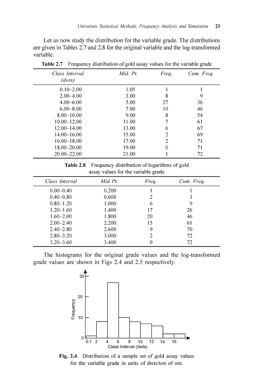
As we see, the distribution
of
gold assay values is far from normal. It
is positively skewed
-the
tail end is to the right. The distribution
of
the
logarithms
of
the 72 gold assay values is approximately normal. (See Tables
2.5 and 2.6 and Figs 2.2 and 2.3)
20
~
c::
Q)
::::>
0-
Q)
u:
10
350
700 1050
1400
Class Interval (inch-dwts)
Fig. 2.2 Distribution
of
a sample set
of
gold accumulation
values in respect
of
lode 0 , gold field I.
30
~
20
c::
Q)
::::>
0-
~
U.
10
4
5
6
Class Interval (in logs)
7
8
Fig. 2.3 Distribution
of
logarithms
of
a sample set
of
gold
accumulation values in respect
of
lode 0 , gold field I.
Univ
ariate Statistical Methods, Frequency Analysis and
Simu
lation 23
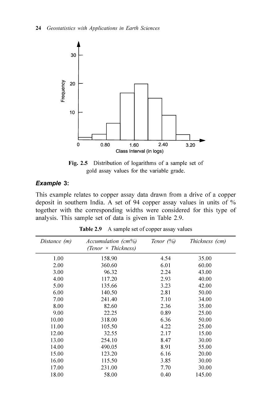
Let us now study the distribution for the variable grade . The distributions
are given in Tables 2.7 and 2.8 for the original variable and the log-transformed
variable.
Tab
le 2.7 Frequency distribution
of
gold assay values for the variable grade
Class Interval Mid. Pt. Freq. Cum. Freq.
(dwts)
0.10
-2
.00
1.05
I I
2.00--4.00 3.00 8 9
4.00-6.00
5.00
27
36
6.00
-8
.00
7.00
10 46
8.00
-10.00
9.00 8 54
10.00
-12
.00 11.00
7
61
12.00
-14
.00 13.00
6 67
14.00
-16.00
15.00 2 69
16.00
-18
.00 17.00 2 71
18.00
-20
.00 19.00
0
71
20.00
-22.00
21.00 I 72
Table 2.8 Frequency distribution
of
logarithms
of
gold
assay values for the variable grade
Class Interval Mid Pt. Freq. Cum. Freq.
0.00-0.40
0.200
I I
0.40-0
.80 0.600 2 3
0.80-1 .20
1.000 6 9
1.20-1 .60 1.400 17 26
1.60
-2
.00
1.800 20 46
2.00
-2.40
2.200 15 61
2.40
-2
.80 2.600
9 70
2.80
-3
.20
3.000 2
72
3.20
-3
.60
3.400 0
72
The histograms for the original grade values and the log-transformed
grade values are shown in Figs 2.4 and 2.5 respectively.
30
20
~
<:
Q)
:>
tr
Q)
u:
10
0 lL---'--
-'-
_
.!...-
--'--
-'-
_
.!...-
--'--
-'-
-
....
0.1 2 4 6 8 10 12 14 16
Class Interval (dwts)
Fig. 2.4 Distribution
of
a sample set
of
gold assay values
for the variable grade in units
of
dwts/ton
of
ore.
24 Geostatistics with Applications in Earth Sciences
30
~
20
c:
Q)
::l
l:T
~
U.
10
o
0.80 1.60 2.40
Class Interval (in logs)
3.20
Fig. 2.5 Distribution
of
logarithms
of
a sample set
of
gold assay values for the variable grade .
Example 3:
This example relates to copper assay data drawn from a drive
of
a copper
deposit in southern India. A set
of
94 copper assay values in units
of
%
together with the corresponding widths were considered for this type
of
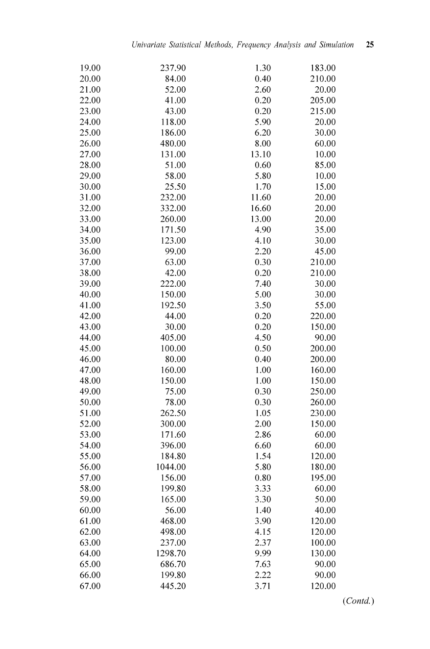
analysis. This sample set
of
data is given in Table 2.9.
Table 2.9 A sample set
of
copper assay values
Distance (m) Accumulation (cm%) Tenor (%) Thickness (em)
(Tenor
x Thickness)
1.00
158.90 4.54
35.00
2.00 360.60 6.01 60.00
3.00 96.32 2.24 43.00
4.00 117.20 2.93 40.00
5.00 135.66
3.23 42.00
6.00
140.50 2.81
50.00
7.00
241.40 7.10 34.00
8.00 82.60 2.36 35.00
9.00 22.25 0.89 25.00
10.00 318.00 6.36 50.00
11
.00 105.50 4.22 25.00
12.00 32.55 2.17 15.00
13.00 254.10 8.47 30.00
14.00 490.05 8.91
55.00
15.00 123.20 6.16 20.00
16.00 115.50
3.85 30.00
17.00 231.00
7.70 30.00
18.00
58.00 0.40
145.00
Univ
ariate Statistical Methods, Frequency Analysis and
Simu
la
tion
25
19.00 237.90
1.30
183.00
20.00 84.00
0040
210.00
21.00 52.00 2.60 20.00
22.00 41.00 0.20 205.00
23.00 43.00 0.20 215.00
24.00
11
8.00 5.90 20.00
25.00 186.00
6.20 30.00
26.00 480.00
8.00 60.00
27.00
131.00
13.10 10.00
28.00 51.00 0.60 85.00
29.00 58.00 5.80 10.00
30.00 25.50 1.70 15.00
31.00 232.00 11.60 20.00
32.00 332.00 16.60 20.00
33.00
260.00 13.00 20.00
34.00 171.50 4.90 35.00
35.00 123.00 4.10 30.00
36.00 99.00 2.20 45.00
37.00 63.00 0.30
210.00
38.00
42.00 0.20 210.00
39.00
222.00
7040
30.00
40.00 150.00 5.00 30.00
41.00 192.50 3.50 55.00
42.00 44.00 0.20 220.00
43.00
30.00
0.20 150.00
44.00 405.00 4.50
90.00
45.00 100.00
0.50
200.00
46.00 80.00
0040
200.00
47.00 160.00 1.00 160.00
48.00 150.00
1.00
150.00
49.00 75.00 0.30 250.00
50.00 78.00 0.30 260.00
51.00 262.50
1.05
230.00
52.00 300.00 2.00 150.00
53.00 171.60 2.86 60.00
54.00 396.00 6.60 60.00
55.00
184.80 1.54 120.00
56.00
1044.00
5.80
180.00
57.00
156.00
0.80
195.00
58.00 199.80 3.33 60.00
59.00 165.00 3.30 50.00
60.00 56.00
l AO 40.00
61.00 468.00 3.90 120.00
62.00 498.00 4.15 120.00
63.00 237.00 2.37 100.00
64.00 1298.70
9.99
130.00
65.00 686.70 7.63 90.00
66.00
199.80 2.22
90.00
67.00
445.20 3.71 120.00
(Contd.)
