Roff D.A. Modeling Evolution: An Introduction to Numerical Methods

Подождите немного. Документ загружается.

Pop[Igen,1:4]<- n[1:4] # Store cohorts

Pop[Igen,5] <- sum(n) # Store total population size

Obs.lambda[Igen,] <- Pop[Igen,]/Pop[Igen-1,] # Store observed

lambda

} # End of Igen loop

# Print out observed lambda in last generation and ratio

print(c(Obs.lambda[Maxgen], Obs.lambda[Maxgen]/Lambda))

par(mfrow¼c(2,2)) # Make 2x2 layout of plots

Generation <- seq(from¼1, to¼Maxgen) # Vector of generation

number

# Plot population and cohort trajectories

ymin <- min(Pop); ymax <- max(Pop) # get minimum and maximum pop

sizes

plot( Generation, Pop[,1], type¼’l’,ylim¼c(ymin,ymax),

ylab¼’Population and cohort sizes’) # Cohort 1

for( i in 2:4) {lines(Generation, Pop[,i]) } # Cohorts 2-4

lines(Generation, Pop[,5], lty¼2) # Total population

# Plot log of population and cohort trajectories

# Log zero is undefined so remove these

x <- matrix(Pop,length(Pop),1) # Convert to one dimensional

matrix

ymin <- min(log(x[x!¼0])) # minimum log value

ymax <- max(log(Pop)) # get minimum and maximum pop sizes

plot( Generation, log(Pop[,1]), type¼’l’, ylim¼c(ymin,ymax),

ylab¼’log Sizes’)

for(i in 2:4) {lines(Generation, log(Pop[,i]))}

lines(Generation, log(Pop[,5]), lty¼2) # Total population

# Plot Observed lambdas

plot(Generation, Obs.lambda[,1], type¼’l’, ylab¼’Lambda’)

for( i in 2:4) {lines(Generation, Obs.lambda[,i])}

lines(Generation, Obs.lambda[,5], lty¼2) # Total population

# Plot observed r

plot(Generation, log(Obs.lambda[,1]), type¼’l’, ylab¼’r’)

for( i in 2:4) {lines(Generation, log(Obs.lambda[,i]))}

lines(Generation, log(Obs.lambda[,5]), lty¼2)

# Total population

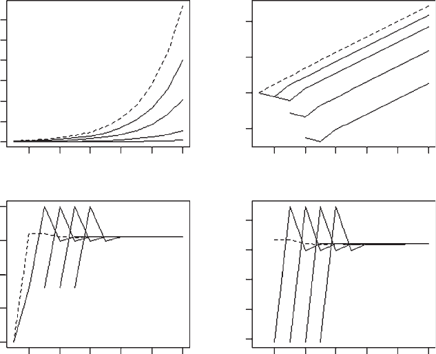
OUTPUT: (Figure 3.1)

168 MODELING EVOLUTION

> print(c(Obs.lambda[Maxgen], Obs.lambda[Maxgen]/Lambda))

[1] 1.5516186þ0i 0.9999971þ0i

The simulation shows that the population quickly reaches a stable age distribu-

tion, shown by the linearity of the plot of log(population or cohort size) on time

and the constancy of the observed l (Figure 3.1).

3.1.2 Modeling evolution using the Leslie matrix

Because the population quickly reaches a stable age distribution and there is no

density-dependence the methods presented in Chapter 2 can be used to analyse

models deﬁned by a Leslie matrix. However, because of the ease with which l or r

(¼ log

l) is calculated from a Leslie matrix, a matrix approach can sometimes be a

more easily programmed method than those used in Chapter 2. Scenario 1 gives

an example of ﬁnding the optimal life history using the Leslie matrix compared to

the approach used in Chapter 2.

Generation Generation

GenerationGeneration

24681012 24681012

2468101224681012

Lambda

Population and cohort sizes

Log Sizes

0.0

–0.2 0.0 0.2 0.4 0.6

–2 0 2 4

0 2040 6080 120

0.5 1.0 1.5 2.0

Figure 3.1 Trajectories of cohort (solid lines) and population sizes (dotted line) and the

observed values of l and

INVASIBILITY ANALYSIS 169

3.1.3 Stage-structured models

In many cases a life cycle is better classiﬁed according to stages rather than

ages: for example, the transition from juvenile to adult is probably more frequent-

ly dependent on passing some size-threshold than a particular age. Suppose we

have a population in which maturity depends upon reaching a minimum size,

after which there are two adult stages. The two adult stages differ and passage

from one to another is also size dependent (e.g., in the ﬁrst adult stage males

might be too small to compete for territories and adopt a satellite strategy. Note

that in this case the symbol F refers to reproductive success). The three transition

equations are

1;tþ1

¼ P

1;t

þ F

2;t

þ F

3;t

2;tþ1

¼ S

1;t

þ P

2;t

3;tþ1

¼ S

2;t

ð3:7Þ

where P

is the surviving proportion that remain in the ith stage and S

is the

proportion that pass from stage i and survive to the next stage. These equations

can be converted into the matrix

1;tþ1

2;tþ1

3;tþ1

0 S

1;t

2;t

3;t

ð3:8Þ

There is no fundamental mathematical difference between age and stage-structured

models and the latter can be analyzed using the “Fisherian” optimality approach.

Difﬁculties arise when ﬁtness is density-dependent, a topic to which we now turn.

3.1.4 Adding density-dependence

The Leslie matrix or its stage-based analogue can be readily modiﬁed to accommo-

date density-dependent effects. There are many ways that a density-dependent

effect can be entered, for example, fertility might only be affected or survival or

both. Only one age class might be affected or the effect spread over several or all

age classes. Two common functions are the Beverton–Holt function and the Ricker

function (both named after the ﬁsheries biologists who suggested it). The Bever-

ton–Holt function is compensatory in that it progresses smoothly to an asymptotic

value, whereas the Ricker function is overcompensatory in that for some portion

of the curve N

tþ1

is less than N

. The standard forms of these two models for an

unstructured population are

tþ1

¼ N

1 þ c

Beverton  Holt

tþ1

¼ N

bN

Ricker

ð3:9Þ

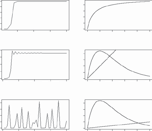
The Beverton–Holt model asymptotes at an equilibrium population, whereas the

Ricker model can equilibrate, cycle, or show chaotic behavior (Figure 3.2). In

applying these functions the population size terms immediately adjacent to the

170 MODELING EVOLUTION

Generation, t

N(t)

N(t+1)

N(t)

20,000 40,000

20,000

40,000

1,000 3,000

20,00040,000

1,000

3,000

20,000 40,000

10 20 30 40

010203040

0 2,000 4,000 6,000 8,000 10,000

2015105

1,000 2,000 3,000 4,000 5,000

Figure 3.2 Examples of population trajectories for the Beverton–Holt (ﬁrst row) and

Ricker models. Depending on parameter values, the Ricker model may reach a stable

equilibrium (second row), or show cyclical behavior (not shown) or chaotic behavior (third

row). Plots on the right show the change in population size as a function of the

previous population. The R coding to produce these plots is as follows:

rm(list=ls()) # Clear workspace

par(mfrow=c(3,2)) # Divide page into 6 panels

BH.FUNCTION <- function(n,c1,c2) {c1/(1+c2*n)}

RICKER.FUNCTION <- function(n, ALPHA, BETA) {ALPHA*exp

(-BETA*n)}

################### MAIN PROGRAM ###################

########## Beverton Holt function ##########

c1 <- 100; c2 <- 2*10^-3 # B-H parameters

# Plot N(t) on t

Maxgen <- 20; N.t <- matrix(0,Maxgen); N.t[1] <- 1

for ( i in 2:Maxgen)

{N.t[i] <- N.t[i-1]*BH.FUNCTION(N.t[i-1], c1,c2)}

plot(seq(from=1, to=Maxgen), N.t, xlab = ’Generation, t’, ylab

=’N(t)’,type=’l’)

# Plot N(t+1) on N(t)

MaxN <- 5000; N.t <- matrix(seq(from=1, to=MaxN))

N.tplus1 <- N.t*apply(N.t,1,BH.FUNCTION, c1,c2)

(cont'd)

INVASIBILITY ANALYSIS 171

equality sign are replaced by fertility and/or survival terms. Thus if fertility in the

previously described Leslie matrix is modiﬁed by a Ricker density dependent

function that affects all ages we have

0:8ae

bN

1:2ae

bN

1:0ae

bN

0ae

bN

0:80 00

00:400

000:25 0

ð3:10Þ

where N

may be the total population size or some particular set of ages (see

example below). How one introduces the density-dependent function is deter-

mined by the biological assumptions. Similarly, the particular density-dependent

function is a function of the particular biological scenario envisaged. If one wishes

to do a general analysis, both functions, with a range of parameter values, should

be tried. Another suggested density-dependent function is the Usher function:

1 þ e

aNþb

ð3:11Þ

which produces a sigmoidal growth curve. Benton and Grant (1999) modiﬁed this

function to produce a gradual or sudden onset of density-dependence:

1 þ e

1:25bN

 50; 000b gradual onset

1 þ e

12:5bN

 500; 000b sudden onset

ð3:12Þ

Fig 3.2 (cont'd)

plot(N.t, N.tplus1, xlab = ’N(t)’, ylab=’N(t+1)’, type=’l’)

########## Ricker function ##########

ALPHA <-c(6, 60); BETA <- .0005 # Parameter values

# Plot N(t) on t for 2 values of ALPHA

Maxgen <- 40

for (j in 1:2)

{

N.t <- matrix(0,Maxgen,1); N.t[1] <- 1

for ( i in 2:Maxgen)

{N.t[i]<- N.t[i-1]*RICKER.FUNCTION(N.t[i-1], ALPHA[j], BETA)}

plot(seq(from=1, to=Maxgen), N.t, xlab = ’Generation, t’, ylab

=’N(t)’, type=’l’)

# Plot N(t+1) on N(t)

MaxN <- 10000; N.t <- matrix(seq(from=1, to=MaxN))

N.tplus1 <- N.t*apply(N.t, 1, RICKER.FUNCTION, ALPHA[j],BETA)

plot(N.t, N.tplus1, xlab=’N(t)’, ylab=’N(t+1)’, type=’l’)

lines(N.t, N.t)

} # End of j loop

172 MODELING EVOLUTION

where b ¼2  10

5

. None of the above equations are sacrosanct and in the absence

of detailed information any function that produces a density-dependent effect

might be tried. In general, the Beverton–Holt and Ricker functions do cover a wide

range of behaviors and are reasonable functions to use.

A simple example of a stage structured model that includes density-dependence

is that for Tribolium spp. proposed by Dennis et al. (1995) and further analyzed by

Grant and Benton (2003). The life cycle of the beetle is divided into three stages,

larval, pupal, and adult with transitions between stages governed by the following

assumptions:

1. The number of larvae at time t þ 1, L

t þ 1

is determined by the number of adults

at time t, A

, the rate at which eggs are cannibalized by adults, c

A.eggs

, and the

rate of cannibalization by the larvae, c

L.eggs

. These effects can be modeled by a

Ricker function.

tþ1

¼ bA

ðc

A:eggs

þc

L:eggs

ð3:13Þ

where b is a constant.

2. The number of pupae that survive to time t þ 1is

tþ1

¼ L

ð3:14Þ

where S

is the survival probability of non-cannibalized larvae.

3. The number of adults is a function of the number of pupae that are canniba-

lized by the adults (a Ricker function) and the survival of adults (S

tþ1

¼ P

c

A:pupae

þ A

ð3:15Þ

These three equations can be written in matrix form as

tþ1

00be

ðc

A:eggs

þc

L:eggs

0 e

c

A:pupae

ð3:16Þ

3.1.5 Estimating ﬁtness

If density-dependence is not a function of the trait of interest and the population

is stable then an appropriate measur e of ﬁtness is R

, which will generally be

much easier to evaluate than using an invasibility approach (see Scenario 2). The

operational deﬁnition of ﬁtness for invasibility analys is is the ability of a novel

clone (the invader) to invade a resident population. However, this does mean

that the invader will replace the resident population as it could coexist with the

resident. The ﬁtness of the invader is the long-term growth rate of the invader

population, which can be e quated to the dominant Lyapunov exponent of the

matrix. In most cases relevant to this book this exponent, also called the invasion

exponent, has to be estimated by simulation. Two approaches for determining the

equilibrium set of trait variables are pairwise invasibility analysis and multiple

invasibility analysis.

INVASIBILITY ANALYSIS 173

3.1.6 Pairwise invasibility analysis

This is a graphical method that identiﬁes putative Evolutionarily Stable Strategies

(ESS) on a surface comprising the set of combinations of resident and invader trait

values. There are four possible outcomes, diagrammed in Figures 3.3 and 3.4. The

x-axis is the set of trait values for the resident and the y-axis is the same set of trait

values representing the trait values of the invader. For each combination we

estimate the long-term growth rate of the invader. The hypothetical long-term

growth rate of the invader in the stationary resident population is given by

the dominant Lyapunov exponent, called by Rand et al. (1994) the invasion

exponent, #:

# ¼ lim

t!1

ð3:17Þ

Because of the small population size of the invader population, the invasion

exponent can be estimated by assuming that the invader population will either

increase or decrease exponentially (at least measured over a sufﬁcient time

period):

tþ1

¼ N

invader

¼ N

invader

lnN

tþ1

¼ lnN

þ t lnl

invader

ð3:18Þ

Thus after some speciﬁed number of iterations the growth rate of the invader

population, #, can be estimated from a linear regression of log(invader population

size) on generation.

Two contour lines are shown on the invasibility plots of Figure 3.3. Both lines

denote the set of combinations at which the growth rate of the invader is zero.

Obviously when the parameter value of the invader is the same as that of the

resident then the invader will neither increase nor decrease: this is the x ¼ y line

shown in the plots. Now consider a trait combination that lies very close to the

origin but above the line of equality: at this point the growth rate of the invader is

positive and it increases in frequency and eventually becomes the resident popu-

lation. For a combination that lies in the upper right of the plots the growth rate of

the invader is negative and it cannot penetrate the resident population. Thus at

some combinations other than x ¼ y the growth rate of the invader must equal

that of the resident population. The point at which this second zero isocline

crosses the line of equality is the putative ESS. Several such points could exist or

there could be zero isoclines that do not intersect the line of equality (e.g., see

White et al. [2006]). Whether the putative ESS is a stable ESS (termed a conver-

gence stable ESS) or an unstable equilibrium depends on the shape of the second

zero isocline: if the slope of the second isocline is greater than 90



as measured in

relation to the x and y-axes (see top plots in Figure 3.3) the intersection is an ESS,

otherwise the equilibrium is unstable and subject to invasion (bottom panels of

Figure 3.3). The plot on the left of Figure 3.3 shows a case in which the putative ESS

is a convergence stable ESS, while that on the right shows a case in which the

intersection deﬁnes an unstable equilibrium termed an evolutionary branching

174 MODELING EVOLUTION

Trait value of resident

Invader

successful

Invader

fails

Invader

successful

Invader

fails

Trait value of invader

Elasticity

Invasion exponent

Trait value of resident

Trait value of invader

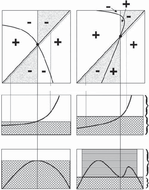
Figure 3.3 Hypothetical examples of pairwise invasibility plots (top panels) in which there

is convergence but not necessarily an ESS. The panels on the left show a convergence stable

ESS and those on the right show an evolutionary branching point. A “+” denotes a positive

long‐term growth rate of the invader population (i.e., invasion successful) and a “−” indicates

a negative long‐term growth rate (i.e., invasion unsuccessful). The dotted lines paralleling the

x = y line indicate the values used in the elasticity analysis and the vertical dotted lines show

examples of the elasticity values obtained at those points. The shaded areas indicate the

zones that are relevant for plotting the invasion exponent of the invader against the

putative ESS value of the resident as shown in the bottom panels. Panels below the ﬁrst row

show the elasticity analyses. In the middle panels the trait value of the invader is set at some

fraction slightly smaller than 1 (e.g., 0.995) of the trait value of the resident. This analysis is

used to determine the putative ESS value. In the bottom panels the trait value of the

resident is set at the putative ESS. This analysis determines if the putative ESS value is

resistant to invasion. The cross‐hatched areas indicate those resident–invader combinations

which lead to extinction of the invader. The horizontal hatched areas indicate trait values

for which invasion occurs when the resident population is at its putative ESS. In the left‐

hand column there are no values for which invasion is successful when the resident

population is at the putative ESS, whereas in the right‐hand plot there are values for which

invasion is successful.

INVASIBILITY ANALYSIS 175

Trait value of invader

Trait value of resident

Trait value of invader

Elasticity

Invasion exponent

Invader

successful

Invader

fails

Invader

successful

Invader

fails

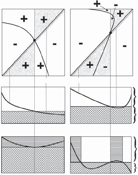
Figure 3.4 Hypothetical examples of pairwise invasibility plots (top panels) in which there

is neither convergence nor a stable ESS. The panels on the right show an invasible repellor

and those on the left show a Garden‐of‐Eden ESS. A “+” denotes a positive long‐term

growth rate of the invader population (i.e., invasion successful) and a “−” indicates a negative

long‐term growth rate (i.e., invasion unsuccessful). The dotted lines paralleling the x = y line

indicate the values used in the elasticity analysis and the vertical dotted lines show examples

of the elasticity values obtained at those points. The shaded areas indicate the zones that

are relevant for plotting the invasion exponent of the invader against the putative ESS value

of the resident as shown in the bottom panels. Panels below the ﬁrst row show the elasticity

analyses. In the middle panels the trait value of the invader is set at some fraction slightly

smaller than 1 (e.g., 0.995) of the trait value of the resident. This analysis is used to

determine the putative ESS value. In the bottom panels the trait value of the resident is set

at the putative ESS. This analysis determines if the putative ESS value is resistant to invasion.

The cross‐hatched areas indicate those resident‐invader combinations which lead to

extinction of the invader. The horizontal hatched areas indicate trait values for which

invasion is indicated by both the analysis of elasticity with respect to the trait value of the

resident (middle panels) and with respect to the trait value of the invader (bottom panels).

In both cases there are combinations from both the elasticity and invasion exponent plots

for which invasion is successful.

176 MODELING EVOLUTION

point. In theory the ESS is not resistant to mutants and polymorphisms will occur

(however, see Scenario 5 of Chapter 4, in which the “unstable” ESS of Scenario 3 of

this chapter is stable when parameters are inherited according to a quantitative

genetic model). The plot of elasticity versus the trait value of the resident shows

that there is convergence but the invasion exponent plotted against the trait value

of the invader shows that invasion is possible in the rightmost scenario. There are

two other possible pairwise invasibility plots, obtained if the areas deﬁning the

positive and negative growth of the invader are reversed (Figure 3.4). In both cases

the elasticity plotted against the trait value of the resident shows that there is no

convergence and the invasion exponent versus the trait value of the invader

shows that invasion is possible in both scenarios. The scenario on the left is

termed an invasibility repellor and that on the right a Garden-of-Eden ESS.

Suppose the trait under study, say X, can reasonably range from X

min

to X

max

.To

produce a pairwise invasibility plot we proceed as follows:

Step 1: Divide X

min

to X

max

. into N

inc

increments. This set of values will be applied

to residents and invaders: for example, in R

X.Resident <- seq(from¼X.min, to¼X.max, length¼N.inc)

X.Invader <- X.residents

Step 2: Create the set of all combinations for resident and invader types. This can

be done using the R function expand.grid

Combinations <- expand.grid(X.Resident, X.Invader)

Step 3: For each combination calculate the population growth rate of the invader

entering a resident population. If this growth rate is positive then the invader trait

value has a higher ﬁtness than the resident trait value. The calculation of the

invader growth rate will typically be estimated by calling some function, say POP.

DYNAMICS that has the following elements in sequence:

a. The call to function POP.DYNAMICS passes the parameter value, in this case

ALPHA, and the multiplier for the invader parameter value, in this case called

Coeff. These two parameters could be passed as a vector of length 2 or, as done

below, as separate elements.

POP.DYNAMICS <- function(ALPHA, Coeff)

ALPHA.resident <- ALPHA # Alpha for resident

ALPHA.invader <- ALPHA*Coeff # Alpha for invader

b. Iteration of population growth of the resident population alone until it has

passed any effects due to initial starting conditions (this does not necessarily mean

that the population will be at equilibrium as it might exhibit cyclical or chaotic

behavior or subject to environmental ﬂuctuations). For example, suppose we run

the resident-only time trace for 50 generations and the time trace after the invader

is introduced for 300 generations. To hold the entire trace, which we might wish

to do for later plotting, we need a matrix of 350 rows.

INVASIBILITY ANALYSIS 177