Richards J.A., Jia X. Remote Sensing Digital Image Analysis: An Introduction

Подождите немного. Документ загружается.

304 11 Image Classiﬁcation Methodologies

of class accuracies will result according to whether the number of correct pixels

for a class is divided by the total number of reference (ground truth) pixels for the

class (the corresponding column sum in Table 11.1) or the total number of pixels

the classiﬁer attributes to the class (the row sum in Table 11.1). Consider class B in

Table 11.1, for example. As noted, 37 of the reference data pixels have been correctly

labelled. This represents 37/40 ≡ 93% of the ground truth pixels for the class. We

interpret this measure, which Congalton and Green (1999) refer to as the Producer’s

accuracy, as the probability that the classiﬁer has labelled the image pixel as B given

that the actual (ground truth) class is B. As a user of a thematic map produced by a

classiﬁer we are more interested in the probability that the actual class is B given that

the pixel has been labelled B (on the thematic map) by the classiﬁer. This is what

Congalton and Green refer to as the User accuracy, and for this example is 37/50 ≡

74%. Thus only 74% of the pixels labelled B on the thematic map are correct, even

though the classiﬁer coped with 93% of the B class reference data. This distinction

is important and leads one to believe that the User accuracy is the ﬁgure that should

most often be adopted.

Some authors prefer to use the kappa coefﬁcient as a measure of map accuracy

(Hudson and Ramm 1987, Congalton and Green 1999). This is deﬁned in terms of

the elements of the error matrix; let these be represented by x

, and suppose the total

number of test pixels (observations) represented in the error matrix is P . Also, let



(i.e. the sum over all columns for row i)



(i.e. the sum over all rows for column j)

then the kappa estimate is deﬁned by

κ =



−



−



Choice of the sample of pixels for accuracy assessment is an important con-

sideration. Perhaps the simplest strategy for evaluating classifer performance is to

choose a set of testing ﬁelds for each class, akin to the training ﬁelds used to esti-

mate class signatures. These testing ﬁelds are also labelled using available reference

data, presumably at the same time as the training areas. After classiﬁcation the accu-

racy of the classifer is determined from its performance on the test pixels. Another

approach, with perhaps more statistical signiﬁcance since it avoids correlated near-

neighbouring pixels, is to choose a random sample of individual pixels across the

thematic map for comparison with reference data. A difﬁculty that can arise with

random sampling in this manner is that it is area-weighted. That is, large classes tend

to be represented by a larger number of sample points than the smaller classes; indeed

some very small classes may not be represented at all. Assessment of the accuracy

11.5 Assessment of Classiﬁcation Accuracy 305

of labelling small classes will therefore be prejudiced. To avoid this it is necessary to

ensure small classes are represented adequately. An approach that is widely adopted

is stratiﬁed random sampling in which the user ﬁrst of all decides upon a set of strata

into which the image is divided. Random sampling is then carried out within each

stratum. The strata could be any convenient area segmentation of the thematic map,

such as gridcells. However the most appropriate stratiﬁcation to use is the actual

thematic classes themselves. Consequently, the user should choose a random sample

within each thematic class to assess the classiﬁcation accuracy of that class.

If one adopts random sampling, stratiﬁed by class, the question that must then be

answered is how many test pixels should be chosen within each class to ensure that

the results entered into the confusion matrix of Table 11.1 are an accurate reﬂection

of the performance of the classiﬁer, and that the percentage correct classiﬁcation so-

derived is a reliable estimate of the real accuracy of the thematic map. To illustrate

this point, a sample of one pixel from a particular class will suggest an accuracy

of 0% or 100% depending on its match to ground truth. A sample of 100 pixels

will clearly give a more realistic estimate. A number of authors have addressed this

problem, using binomial statistics, in the following manner.

Let the pixels from a particular category in a thematic map be represented by the

random variable x that takes on the value 1 if a pixel is correctly classiﬁed and 0

otherwise. Suppose the true map accuracy for that class is θ (which is what we wish

to estimate by sampling). Then the probability of x pixels being correct in a random

sample of n pixels from that class is given by the binomial probability

p(x;n, θ ) =

(1 − θ)

n−x

x = 0, 1,... ,n . (11.1)

Van Genderen et al. (1978) determine the minimum sample size, by noting that if

the sample is too small there is a ﬁnite chance that those pixels selected could all be

labelled correctly (as for example in the extreme situation of one pixel considered

above). If this occurs then a reliable estimate of the map accuracy clearly has not been

obtained. Such a situation is described by x = n in (11.1), giving as the probability

for all n samples being correct

p(n;n, θ ) = θ

Van Genderen et al. have evaluated this expression for a range of θ and n and have

noted that p(n;n, θ ) is unacceptably high if it is greater than 0.05 – i.e. if more than

5% of the time there is a chance of selecting a perfect sample from a population in

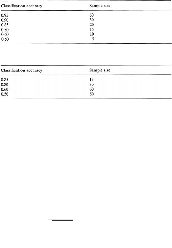
which the accuracy is actually described by θ. A selection of their results is given

in Table 11.2. In practice, these ﬁgures should be exceeded to ensure representative

outcomes are obtained. Van Genderen et al. consider an extension of the results in

Table 11.2 to the case of encountering set levels of error in the sampling, from which

further recommendations are made concerning desirable sample sizes.

Rosenﬁeld et al. (1982) have also determined guidelines for selecting minimum

sample sizes. Their approach is based upon determining the number of samples

required to ensure that the sample mean – i.e. the number of correct classiﬁcations

divided by the total number of samples per category – is within 10% of the population

306 11 Image Classiﬁcation Methodologies

Table 11.2. Minimum sample size necessary per category (after Van Genderen et al. 1978)

Table 11.3. Minimum sample size necessary per category (after Rosenﬁeld et al. 1982)

mean (i.e. the map accuracy for that category) at a 95% conﬁdence level. Again

this is estimated from binomial statistics, although using the cumulative binomial

distribution. Table 11.3 illustrates the results obtained; while these results agree with

Table 11.2 for a map accuracy of 85% the trends about this point are opposite.

This perhaps is not surprising since the two approaches commence from different

viewpoints. Rosenﬁeld et al. are interested in ensuring that the accuracy indicated

from the samples (i.e. sample mean) is a reasonable (constant) approximation of the

actual map accuracy. In contrast, Van Genderen et al. base their approach on ensuring

that the set of samples is representative. Both have their merits and in practice one

may wish to choose a compromise of between 30 and 60 samples per category.

Once accuracy has been estimated through sampling it is important to place some

conﬁdence on the actual ﬁgures derived for each category. In fact it is useful to be

able to express an interval within which the true map accuracy lies (with say 95%

certainty). This interval can be determined from the accuracy estimate for a class

using the expression (Freund, 1992)

−z

α/2

x − nθ

√

nθ(1 −θ)

α/2

= 1 − α (11.2)

where x is the number of correctly labelled pixels in a sample of n;θ is the true map

accuracy (which we currently are estimating in the usual way by x/n) and 1 − α

is a conﬁdence limit. If we choose α = 0.05 then the above expression says that

the probability that (x −nθ)/

√

nθ(1 −θ) will be between ±z

α/2

is 95%; ±z

α/2

are

points on the normal distribution between which 1−α of the population is contained.

For α = 0.05, tables show z

α/2

= 1.960. Equation (11.2) is derived from properties

of the normal distribution; however for a large number of samples (typically 30 or

11.6 Case Study 1: Irrigated Area Determination 307

more) the binomial distribution is adequately represented by a normal model making

(11.2) acceptable. Our interest in (11.2) is seeing what limits it gives on θ. It is shown

readily, at the 95% level of conﬁdence, that the extreme values of θ are given by

x + 1.921 ± 1.960

{

x(n − x)/n + 0.960

}

n + 3.842

(11.3)

As an illustration, suppose x = 294,n = 300 for a particular category. Then ordinar-

ily we would use

x = x/n = 0.98 as an estimate of θ , the true map accuracy for the

category. Equation (11.3) however shows, with 95% conﬁdence, that our estimate of

θ is bounded by

0.9571 <θ<0.9908 .

Thus the accuracy of the category in the thematic map is somewhere between 95.7%

and 99.1%.

This approach has been developed by Hord and Brunner (1976) who produced

tables of the upper and lower limits on the map accuracy as a function of sample size

and sample mean (or accuracy)

x = x/n.

11.5.2

The Leave One Out Method of Accuracy Assessment – Cross Validation

An interesting accuracy assessment method, which does not depend on developing a

testing set of pixels, is the Leave One Out (LOO) approach. It is based on removing

one of the training set of pixels, training the classiﬁer on the remainder and using the

trained classiﬁer to label the pixel left out. That pixel is replaced and another removed

and the process repeated. This is done for all pixels in the training set. The average

classiﬁcation accuracy is then determined. Provided the original training pixels are

representative, this method produces an unbiased estimate of classiﬁcation accuracy

(Landgrebe, 2003).

The Leave One Out method is a special case of cross validation (Duda, Hart and

Stork, 2001) in which the available labelled pixels are divided into k subsets. One

of those subsets is used as the testing data and the remainder aggregated to form the

training set. The process is repeated k times, so that each subset in turn is used as the

testing data and the others for training.

11.6

Case Study 1: Irrigated Area Determination

It is the purpose of this case study to demonstrate a simple classiﬁcation, carried out

using the hybrid strategy of Sect. 11.4. Rather than being based upon iterative clus-

tering and maximum likelihood classiﬁcation it makes use of a single pass clustering

algorithm of the type presented in Sect. 9.6 and a minimum distance classiﬁer as

described in Sect. 8.3.

308 11 Image Classiﬁcation Methodologies

The problem presented was to use classiﬁcation of Landsat Multispectral Scanner

image data to assess the hectarage of cotton crops being irrigated by water from the

Darling River in New South Wales. This was to act as a cross check of area estimates

provided by ground personnel of the New South Wales Water Resources Commission

and the New South Wales Department of Agriculture. More details of the study and

the presentation of some alternative classiﬁcation techniques for this problem will

be found in Moreton and Richards (1984), from which the following sections are

adapted.

11.6.1

Background

Much of the western region of the state of New South Wales in Australia experiences

arid to semi-arid climatic conditions with low average annual rainfalls accompanied

by substantial evapotranspiration. Consequently, a viable crop industry depends to a

large extent upon irrigation from major river systems. Cotton growing in the vicinity

of the township of Bourke is a particular example. With an average annual rainfall

of 360 mm, cotton growing succeeds by making use of irrigation from the nearby

Darling River. This river also provides water for the city of Broken Hill further

downstream and forms part of a major complex river system ultimately that provides

water for the city of Adelaide, the capital of the state of South Australia. The Darling

River itself receives major inﬂows from seasonal rains in Queensland, and in dry

years can run at very low levels or stop ﬂowing altogether, leading to increased

salination of the water supplies of the cities downstream. Consequently, additional

demands on the river made by irrigation must be carefully controlled. In New South

Wales such control is exercised by the issue of irrigation licenses to farmers. It is

then necessary to monitor their usage of water to ensure licenses are not infringed.

This, of course, is the situation in many parts of the world where extensive irrigation

systems are in use.

The water demand by a particular crop is very closely related to crop area, because

most water taken up by a plant is used in transpiration (Keene and Conley, 1980).

As a result, it is sufﬁcient to monitor crop area under irrigation as an indication of

water used. In this example, classiﬁcation is used to provide crop area estimates.

11.6.2

The Study Region

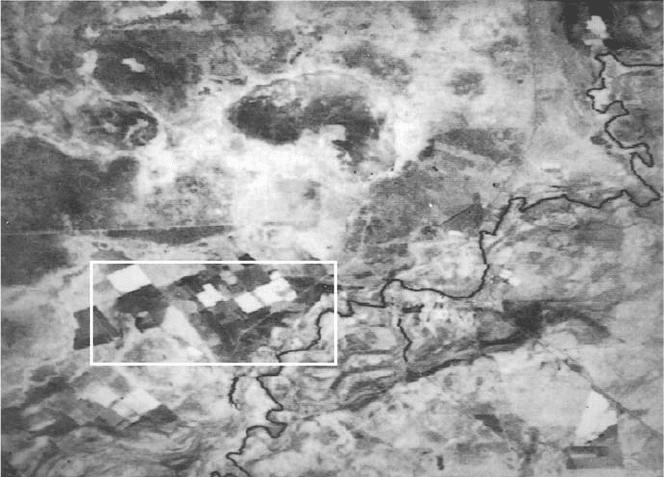
A band 7 Landsat Multispectral Scanner image of the region considered in the study,

consisting of 927 lines of 1102 pixels, is shown in Fig. 11.1. This is a portion of

scene number 30704–23201 acquired in February 1980 (Path 99, Row 81). Irrigated

cotton ﬁelds are clearly evident as bright ﬁelds in the central left and bottom right

regions, as is a further crop in the top right. The township of Bourke is just south of

the Darling River, just right of the center of the image. The white border encloses

a subset of the data, shown enlarged in Fig. 11.2. This smaller region was used for

signature generation.

11.6 Case Study 1: Irrigated Area Determination 309

Fig. 11.1. Band 7 Landsat MSS image of the region of the investigation, showing irrigated

ﬁelds (white). The area enclosed by the white border was used for signature generation.

Reproduced from Photogrammetric Engineering & Remote Sensing. Vol. 50, June 1984

11.6.3

Clustering

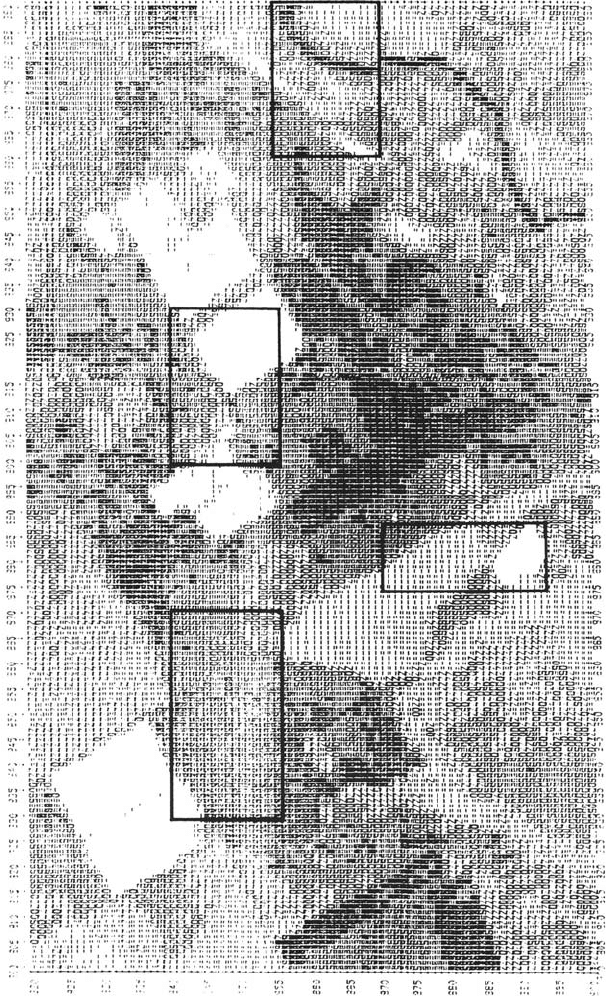
Figure 11.2 shows the location of four regions selected for clustering using the

single-pass algorithm. A ﬁfth clustering region was chosen which partially included

the triangular ﬁeld in the bottom right region of Fig. 11.1. These regions consist

of up to 500 pixels each and were selected so that a number of the irrigated cotton

ﬁelds were included, along with a choice of most of the other major ground covers

thought to be present. These include bare ground, lightly wooded regions, such as

trees along the Darling River, apparently non-irrigated (and/or fallow) crop land, and

a light coloured sand or soil.

Each of the regions shown in Fig. 11.2 was clustered separately. With the pa-

rameters entered into the clustering algorithm, each region generated between ﬁve

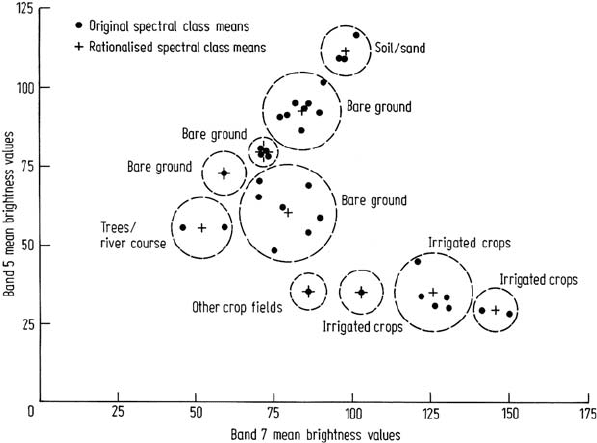
and 11 spectral classes. The centres of the complete set of 34 spectral classes were

then located on a bispectral plot. Sometimes such a plot could be the average of the

visible components of the cluster means (Landsat bands 4 and 5) versus the average

of the infrared components (bands 6 and 7). In this exercise, however, owing to the

well-discriminated nature of the data, a band 5 versus band 7 bispectral plot was used;

moreover, the subsequent classiﬁcation also made use only of bands 5 and 7. This

reduced the cost of the classiﬁcation phase; however, the results obtained suggest

310 11 Image Classiﬁcation Methodologies

Fig. 11.2. Line printer map (band 7) of the region shown enclosed in a white border in Fig. 11.1. Cluster regions are indicated by the

black borders. Reproduced from Photogrammetric Engineering & Remote Sensing, Vol. 50, June 1984

11.6 Case Study 1: Irrigated Area Determination 311

Fig. 11.3. Bispectral plot (band 5 class means versus band 7 class means) showing the orig-

inal 34 cluster centers (spectral classes) generated. Also shown are the class rationalisations

adopted. Original spectral classes within the dotted circles were combined to form a single

class with mean positions indicated. The labels were determined from reference data and

spectral response characteristics. Reproduced from Photogrammetric Engineering & Remote

Sensing, Vol. 50, June 1984

that accuracy was not prejudiced. The band 5 versus band 7 bispectral plot showing

the clustering results is illustrated in Fig. 11.3.

At this stage, it was necessary to rationalize the number of spectral classes and

to associate spectral classes with ground cover types (so-called information classes).

While a sufﬁcient number of spectral classes must be retained to ensure classiﬁ-

cation accuracy, it is important not to have too many, because the number of class

comparisons, and thus the cost of a classiﬁcation, is directly related to this number.

Because the classiﬁer to be employed was known to be of the minimum distance

variety, which implements linear decision surfaces between classes, spectral classes

were merged into approximately circular groups (provided they were from the same

broad cover type) as shown in Fig. 11.3. In this manner, the number of classes was

reduced to ten. Labels were attached to each of those (as indicated in Fig. 11.3)

by comparing cluster maps to black-and-white and color aerial photography, and to

band 7 imagery. The relative band 5 and band 7 brightness values were also employed

for class recognition; ﬁelds under irrigation were evident by their low band 5 values

(30 on a scale of 255, indicating high chlorophyll absorption) accompanied by high

band 7 reﬂectance (100 to 150, indicating healthy, well-watered vegetation).

312 11 Image Classiﬁcation Methodologies

11.6.4

Signature Generation

Signatures for the rationalized spectral classes were generated by averaging the means

of the constituent original set of spectral classes. This was done manually, and is an

acceptable procedure for the classiﬁer used. Minimum distance classiﬁcation makes

use only of class means in assigning pixels and does not take any account of class

covariance data. On the contrary, maximum likelihood classiﬁcation incorporates

both class covariance matrices and mean vectors as signatures, and merging of con-

stituent spectral class signatures to obtain those for rationalized classes cannot readily

be done by hand. Rather, a routine that combines class statistics is required.

The rationalized class means are indicated in Fig. 11.3.

11.6.5

Classiﬁcation and Results

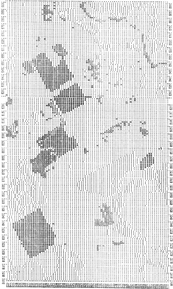
With spectral class signatures determined as above, Fig. 11.1 was checked for crop

ﬁelds that indicated use of irrigation. A classiﬁcation map of the Fig. 11.2 (6,957 ha)

region is shown in Fig. 11.4. Fields under irrigation are clearly discernible by their

shape, as well as by their classiﬁcation. By retaining several other ground-cover

types as separate information classes (rather than giving them all a common symbol

representing “non-irrigated”), other geometric features of interest are evident. For

example, the Darling River is easily seen, as are some neighbouring ﬁelds that are

not irrigated. This was useful for checking the results of the classiﬁcation against

maps and other reference data.

The results of the classiﬁcation agreed remarkably well with ground-based data

gathered by ﬁeld ofﬁcers of the New South Wales Water Resources Commission

and the New South Wales Department of Agriculture. In particular, for a region of

169651 pixels (75,000 ha) within Fig. 11.1, a measure of 803 ha given by the classiﬁer

as being under irrigation agreed to better than 1% with that given by ground data. This

is well within any experimental error that could be associated with the classiﬁcation

and with the uncertainty regarding pixel size (in hectares), and is consistent with

accuracies reported by some other investigators (Tinney et al., 1974).

11.6.6

Concluding Remarks

In general, the combined clustering/supervised classiﬁcation strategy adopted works

well as a means for identifying a reliable set of spectral classes upon which a clas-

siﬁcation can be based. The clustering phase, along with a construction such as a

bispectral plot, is a convenient and lucid means by which to determine the structure

of image data in multispectral space; this would especially apply for exercises that

are as readily handled as those described here. The rationalized spectral classes used

in this case correspond not so much to unimodal Gaussian classes normally asso-

ciated with maximum likelihood classiﬁcation, but rather are a set that match the

11.6 Case Study 1: Irrigated Area Determination 313

Fig. 11.4. Classiﬁcation map of the region of Fig. 11.2 generated using the ORSER software package. Class symbols used are:

∗ irrigated crops; + other crop ﬁelds; × trees/river course; – soil/sand; bare ground. Reproduced from Photogrammetric Engineering

& Remote Sensing, Vol. 50, June 1984