Richards J.A., Jia X. Remote Sensing Digital Image Analysis: An Introduction
Подождите немного. Документ загружается.

264 9 Clustering and Unsupervised Classification
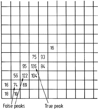
Fig. 9.9. False indication of peaks in a two
dimensional histogram, when the peak detec-
tion algorithm only searches parallel to the
bins
total number of four dimensional bins is now 6×8 ×6 ×6 = 1728. With a 100 ×100
pixel image segment therefore, there are, on the average, 6 pixels per bin which is
probably acceptable (although low) to guarantee that peaks determined represent the
location of real clusters in the data and not artifacts. Clearly resolution is sacrificed
but this is necessary to yield an acceptable clustering by this approach.
The maximum detection algorithm used in this clustering procedure cannot be too
sophisticated otherwise the method becomes too expensive to implement. Usually
it consists of locating bins in which the count is higher than in the neighbouring
bins along the same row and down the same column. For correlated data this can
sometimes lead to false indications of peaks, as depicted in Fig. 9.9, in the vicinity
of true peaks. This will be so particularly for smaller bin sizes. A better maximum
detection procedure is to check diagonal neighbours as well but of course this doubles
the search time.
Clearly this technique is only useful when the dimensionality of the data is low
(just a few spectral bands). Because of the enormous number of bins that would be
generated, and the extreme sparseness of the resulting histogram (see Problem 1.9),
the method is not applicable to hyperspectral data sets.
References for Chapter 9
Cluster analysis is a common tool in many applications that involve large amounts of data.
Consequently source material on clustering algorithms will be found spread over many disci-
plines including numerical taxonomy, the social sciences and the physical sciences. However,
because of the immense volumes of data to be clustered in remote sensing, the range of tech-
niques that can be used is limited largely to those methods presented in this chapter and to their
variations. Some more general treatments however that may be of value include Anderberg
(1973), Hartigan (1975), Tryon and Bailey (1970) and Ryzin (1977).
Problems 265
M.R. Anderberg, 1973: Cluster Analysis for Applications. N.Y. Academic.
G.H. Ball and D.J. Hall, 1965: A Novel Method of Data Analysis and Pattern Classification.
Stanford Research Institute, Menlo Park, California.
G.R. Coleman and H.C. Andrews, 1979: Image Segmentation by Clustering. Proc. IEEE, 67,
773–785.
R.D. Duda, P.E. Hart and D.G. Stork, 2001: Pattern Classification, 2e. N.Y., Wiley.
J.A. Hartigan, 1975: Clustering Algorithms. N.Y., Wiley.
D.J. Kelly, 1983: The Concept of a Spectral Class – A Comparison of Clustering AIgorithms.
M. Eng. Sc. Thesis. The University of New South Wales, Australia.
D.A. Landgrebe and L. Biehl, 1995: An Introduction to MultiSpec. West Lafayette, Purdue
Research Foundation (http: //dynamo.ecn.purdue.edu/∼biehl/MultiSpec
P.A. Letts, 1978: Unsupervised Classification in The Aries Image Analysis System. Proc. 5th
Canadian Symp. on Remote Sensing, 61–71.
T.L. Phillips (Ed.), 1973: LARSYS Version 3 Users Manual. Laboratory for Applications of
Remote Sensing, Purdue University, West Lafayette.
J. van Ryzin, 1977: Classification and Clustering. N.Y., Academic.
R.C. Tryon and D.E. Bailey, 1970: Cluster Analysis, N.Y., McGraw-Hill.
Problems
9.1 Repeat the exercise of Fig. 9.2 but with
(i) two initial cluster centres at (2,3) and (5,6),
(ii) three initial cluster centres at (1,1), (3,3) and (5,5), and
(iii) three initial cluster centres at (2,1), (4,2) and (15,15).
9.2 From a knowledge of how a particular clustering algorithm works it is sometimes possible
to infer the multidimensional spectral shapes of the clusters generated. For example, methods
that depend entirely upon Euclidean distance as a similarity metric would tend to produce
hyperspheroidal clusters. Comment on the cluster shapes you would expect to be generated by
the migrating means technique based upon Euclidean distance and the single pass procedure,
also based upon Euclidean distance.
9.3 Suppose two different techniques have given two different clusterings of a particular set
of data and you wish to assess which of the two segmentations is the better. One approach
might be to evaluate the sum of square errors measure treated in Sect. 9.2. Another could
be based upon covariance matrices. For example it is possible to define an “among clusters”
covariance matrix that describes how the clusters themselves are scattered about the data space,
and an average “within class” covariance matrix that describes the average shape and size of
the clusters. Let these be called Σ
A
and Σ
W
respectively. How could they be used together
to assess the quality of the two clustering results? (See Coleman and Andrews, 1979) Here
you may wish to use measures of the “size” of a matrix, such as its trace or determinant (see
Appendix D).
9.4 Different clustering methods often produce quite different segmentations of the same set
of data, as illustrated in the examples of Figs. 9.3 and 9.6. Yet the results generated for remote
sensing applications are generally usable. Why do you think that is the case? (Hint: Is it related
to the number of clusters generated?)
266 9 Clustering and Unsupervised Classification
9.5 The Mahalanobis distance of (8.13) can be used as the similarity metric for a clustering
algorithm. Invent a possible clustering technique based upon (8.13) and comment on the nature
of the clusters generated.
9.6 Do you see value in having a two stage clustering process say in which a single pass
procedure is used to generate initial clusters and then an iterative technique is used to refine
them?
9.7 Recompute the agglomerative hierarchical clustering example of Fig. 9.7 but use the L1
distance measure in (9.2) as a similarity metric.
9.8 The histogram peak selection clustering technique of Sect. 9.8 has some shortcomings.
One is related to the need to have large spectral bins in the histogram in order to have a
sensible histogram produced when the data dimensionality is high. A consequence is that
fine spectral resolution is sacrificed leading to loss of discrimination of spectral classes that
are very close. Do you think good spectral discrimination could be regained by applying the
technique several times over, on each subsequent occasion clustering just within one of the
clusters found previously? Discuss the details of this approach.
9.9 Consider the two dimensional data shown in Fig. 9.2, and suppose the three pixels at the
upper right form one cluster and the remainder another cluster. Such an assignment might
have been generated by some clustering algorithm other than iterative optimisation. Calculate
the sum of squared error for this new assignment and compare with the value of 16 found in
Fig. 9.2. Comment?
10
Feature Reduction
10.1
Feature Reduction and Separability
Classification cost increases with the number of features used to describe pixel vectors
in multispectral space – i.e. with the number of spectral bands associated with a pixel.
For classifiers such as the parallelepiped and minimum distance procedures this is
a linear increase with features; however for maximum likelihood classification, the
procedure most often preferred, the cost increase with features is quadratic. Therefore
it is sensible economically to ensure that no more features than necessary are utilised
when performing a classification.
Section 8.2.6 draws attention to the number of training pixels needed to ensure
that reliable estimates of class signatues can be obtained. In particular, the number
of training pixels required increases with the number of bands or channels in the
data. For high dimensionality data, such as that from imaging spectrometers, that
requirement presents quite a challenge in practice, so keeping the number of features
used in a classification to as few as possible is important if reliable results are to be
expected from affordable numbers of training pixels.
Features which do not aid discrimination, by contributing little to the separability
of spectral classes, should be discarded. Removal of least effective features is referred
to as feature selection, this being one form of feature reduction. The other is to
transform the pixel vector into a new set of coordinates in which the features that can
be removed are made more evident. Both procedures are considered in some detail
in this chapter.
Feature selection cannot be performed indiscriminantly. Methods must be devised
that allow the relative worths of features to be assessed in a quantitative and rigorous
way. A procedure commonly used is to determine the mathematical separability
of classes; in particular, feature reduction is performed by checking how separable
various spectral classes remain when reduced sets of features are used. Provided
separability is not lowered unduly by the removal of features then those features can
be considered of little value in aiding discrimination.
268 10 Feature Reduction
10.2
Separability Measures
for Multivariate Normal Spectral Class Models
(Adapted in part from Swain and Davis, 1978)
10.2.1
Distribution Overlaps
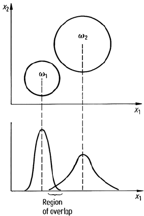
Consider a two dimensional multispectral space with two spectral classes as depicted
in Fig. 10.1. Suppose we wish to see whether the classes could be separated using
only one feature – either x
1
or x
2
. Of course it is not known which feature offers the
best prospects a priori. This is what has to be determined by a measure of separability.
Consider an assessment of x
1
. The spectral classes in the x
1
‘subset’ or subspace are
shown in the figure whereupon some overlap of the single dimensional distributions
is indicated. If the distributions are well separated in the x
1
dimension then clearly
the overlap will be small and it would be unlikely that a classifier would make an
error in discriminating between them on the basis of that feature alone. On the other
hand for a large degree of overlap substantial classifier error would be expected. The
usefulness of the x
1
feature subset therefore can be assessed in terms of the overlap
of the distributions in that domain, or more generally, in terms of the similarity of
the distributions as a function of x
1
alone.
Consider now an attempt to quantify the separation between a pair of probability
distributions (as models of spectral classes) as an indication of the degree of overlap.
Clearly distance between means is insufficient since overlap will also be influenced
by the standard deviations of the distributions. Instead, a combination of both the
Fig. 10.1. Two dimensional multispectral space
showing a hypothetical degree of separation pos-
sible in a single dimension subspace (in which
class densities are shown)
10.2 Separability Measures for Multivariate Normal Spectral Class Models 269
distance between means and a measure of standard deviation is required. Moreover
this must be a vector-based measure in order to be applicable to multidimensional
subspaces. Several such measures are available; only those commonly encountered
in connection with remote sensing data are treated in this chapter. Others may be
found in books on statistics that treat similarities in probability distributions. These
measures are all referred to as measures of separability which implies the ease with
which patterns can be correctly associated with their classes using statistical pattern
classification.
10.2.2
Divergence
10.2.2.1
A General Expression
Divergence is a measure of the separability of a pair of probability distributions that
has its basis in their degree of overlap. It is defined in terms of the likelihood ratio
L
ij
(x) = p(x|ω
i
)/p(x|ω
j
)
where p(x|ω
i
) and p(x|ω
j
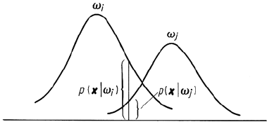
) are the values of the ith and jth spectral class probability
distributions at the position x. These are shown in an overlap region in Fig. 10.2
whereupon it is evident that L
ij
(x) is a measure of ‘instantaneous’ overlap. Clearly
for very separable spectral classes L
ij
(x) = 0or∞ for all x.
It is of value to choose the logarithm of the likelihood ratio, viz
L
ij
= ln p(x|ω
i
) − ln p(x|ω
j
),
by means of which the divergence of the pair of class distribution is defined as
d
ij
= E{L
ij
(x)|ω
i
}+E{L
ji
(x)|ω
j
} (10.1)
where E{} is the expectation operator defined for continuous distributions as
E{L
ij
(x)|ω
i
}=
x
L
ij
(x)p(x|ω
i
) dx.
This is the average or expected value of the likelihood ratio with respect to all patterns
Fig. 10.2. Definition of the probabil-
ities used in the likelihood ratio
270 10 Feature Reduction
in the ith spectral class. Similarly for E{L
ji
(x)|ω
j
}. From (10.1) it can be seen that
d
ij
=
x
{p(x|ω
i
) − p(x|ω
j
)} ln
p(x|ω
i
)
p(x|ω
j
)
dx
from which a number of properties of divergence can be established. For example it
is always positive and also d
ji
= d
ij
, as should be the case – i.e., it is symmetric.
Moreover, if p(x|ω
i
) = p(x|ω
j
) for all x then d
ij
= d
ji
= 0 – in other words there
is no divergence (or difference) between a distribution and itself.
For statistically independent features (i.e., spectral components) x
1
,x
2
, ···,
x
N
then
p(x|ω
i
) =
N
"
n=1
p(x
n
|ω
i
)
which leads to
d
ij
(x) =
N
n=1
d
ij
(x
n
).
Since divergence is never negative it follows therefore that
d
ij
(x
1
, ···x
n
,x
n+1
)>d
ij
(x
1
, ···x
n
).
In other words, divergence never decreases as the number of features is increased.
The material to this point has been general, applying to any multivariate spectral
class model.
10.2.2.2
Divergence of a Pair of Normal Distributions
Since spectral classes in remote sensing image data are modelled by multidimen-
sional normal distributions it is of particular interest to have available the specific
form of (10.1) when p(x|ω
i
) and p(x|ω
j
) are normal distributions with means and
covariances of m
i
,Σ
i
and m
j
,Σ
j
respectively.
By substitution of the full expressions for the normal distributions it can be
shown that
d
ij
=
1
2
T
r
(Σ
i
− Σ
j
)(Σ
−1
j
− Σ
−1
i
)
+
1
2
T
r
(Σ
−1
i
+ Σ
−1
j
)(m
i
− m
j
)(m
i
− m
j
)
t
= Term 1 + Term 2.
(10.2)
where T
r
{} is the trace of the subject matrix. Note that Term 1 involves only covari-
ances whereas Term 2 is the square of a normalised (by covariance) distance between
the means of the distributions.
Equation (10.2) gives the divergence between a pair of spectral classes that are
normally distributed. Should there be more than two spectral classes, as is generally

10.2 Separability Measures for Multivariate Normal Spectral Class Models 271
the case, all pairwise divergences need to be checked to see whether a particular
feature subset gives sufficiently separable data. An average indication of separability
is then given by computing the average divergence
d
ave
=
M
i=1
M
j=i+1
p(ω
i
)p(ω
j
)d
ij
(10.3)
where M is the number of spectral classes and p(ω
i
), p(ω
i
) are the class prior
probabilities.
10.2.2.3
Use of Divergence for Feature Selection
Consider the need to select the best three discriminating channels for Landsat mul-
tispectral scanner data, for an image in which only three spectral classes exist. The
pairwise divergence between each pair of spectral classes would therefore be deter-
mined for all combinations of three out of four channels or bands. The feature subset
chosen would be that which gives the highest overall indication of divergence –
presumably this would be the highest average divergence. Table 10.1 illustrates the
number of divergence calculations required for such an example.
In general, for M spectral classes, N total features, and a need to select the best
n feature subset, the following set of pairwise divergence calculations are necessary,
leaving aside the need finally to compute the average divergence for each subset.
First there are
N
C
n
possible combinations of n features from the total N , and for
each combination there are
M
C
2
pairwise divergence measures to be computed. For
a complete evaluation therefore
N
C
n
·
M
C
2
measures of pairwise divergence have to be calculated. To assess the best 4 of 7
Landsat Thematic Mapper bands for an image involving 10 spectral classes then
7
C
4
·
10
C
2
= 1575
divergence values have to be computed. Inspection of (10.2) shows each divergence
calculation to be considerable. This, together with the large number required in
a typical problem, makes the use of divergence to check separability and indeed
separability analysis in general, an expensive process computationally.
Table 10.1. Divergence calculation table
* Entries to be calculated
272 10 Feature Reduction
10.2.2.4
A Problem with Divergence
As spectral classes become further removed from each other in multispectral space,
the probability of being able to classify a pattern at a particular location moves
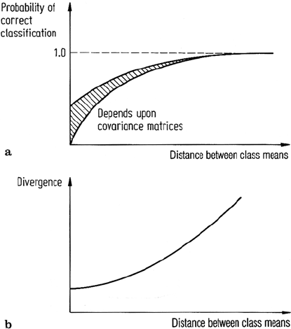
asymptotically to 1.0 as depicted in Fig. 10.3a. If divergence is similarly plotted it
will be seen from its definition that it increases quadratically with separation be-
tween spectral class means as depicted in Fig. 10.3b. This behaviour unfortunately
is quite misleading if divergence is to be used as an indication of how successfully
patterns in the corresponding spectral classes could be mutually discriminated or
classified. It implies, for example, that at large separations, further small increases
will lead to vastly better classification accuracy whereas in practice this is not the
case as observed from the very slight increase in probability of correct classifica-
tion implied by Fig. 10.3a. Moreover, outlying, easily separable classes will weight
average divergence upwards in a misleading fashion to the extent that sub-optimal
reduced feature subsets might be indicated as best, as illustrated in Swain and Davis
(1978). This problem renders divergence, as it is presently defined, to be unsuitable
and indeed unsatifactory. The Jeffries-Matusita distance in the next section does not
suffer this drawback.
Fig. 10.3. a Probability of correct classification as a function of spectral class separation;
b divergence as a function of spectral class separation
10.2 Separability Measures for Multivariate Normal Spectral Class Models 273
10.2.3
The Jeffries-Matusita (JM) Distance
10.2.3.1
Definition
The JM distance between a pair of probability distributions (spectral classes) is
defined as
J
ij
=
x
{
√
p(x|ω
i
) −
√
p(x|ω
j
)}
2
dx (10.4)
which is seen to be a measure of the average distance between the two class density
functions (Wacker, 1971). For normally distributed classes this becomes
J
ij
= 2
1 − e
−B
(10.5)
in which
B =
1
8
(m
i
− m
j
)
t
#
Σ
i
+ Σ
j
2
$
−1
(m
i
− m
j
)
+
1
2
ln
#
|(Σ
i
+ Σ
j
)/2|
|Σ
i
|
1/2
|Σ
j
|
1/2
$
(10.6)
which is referred to as the Bhattacharyya distance (Kailath, 1967).
It is of interest to note that the first term in B is akin to the square of the normalised
distance between the class means. The presence of the exponential factor in (10.5)
gives an exponentially decreasing weight to increasing separations between spectral
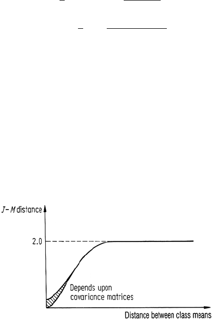
classes. If plotted as a function of distance between class means it shows a saturating
behaviour not unlike that expected for the probability of correct classification, as
seen in Fig. 10.4.
It is asymptotic to 2.0 so that a JM distance of 2.0 between spectral classes would
imply classification of pixel data into those classes, (assuming they were the only
two) with 100% accuracy. This saturating behaviour is highly desirable since it does
not suffer the difficulty experienced with divergence.
Fig. 10.4. Jeffries-Matusita
distance as a function of sep-
aration between spectral class
means
