Richards J.A., Jia X. Remote Sensing Digital Image Analysis: An Introduction

Подождите немного. Документ загружается.

8.9 Non-parametric Classiﬁcation: Geometric Approaches 233

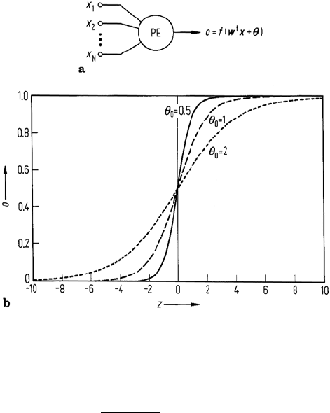
Fig. 8.19. a Neural network processing element. b Plots of (8.38) for various θ

thresholding in a soft or asymptotic sense and be differentiable. The most commonly

encountered expression is

f(z) =

1 + e

−z/θ

(8.38)

where the argument z is w

x+θ as seen in (8.37) and θ

is a constant. This approaches

1 for z large and positive and 0 for z large and negative and is thus asymptotically

thresholding. It is important to recognise that the outcome of the product w

x is a

simple scalar; when plotted with θ = 0, (8.38) appears as shown in Fig. 8.19b. For

very small the activation function approaches a thresholding operation. Usually

= 1.

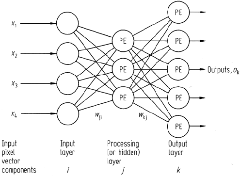
A neural network for use in remote sensing image analysis will appear as shown

in Fig. 8.20, being a layered classiﬁer composed of processing elements of the type

shown in Fig. 8.19a. It is conventionally drawn with an input layer of nodes (which

has the function of distributing the inputs to the processing elements of the next layer,

and scaling them if necessary) and an output layer from which the class labelling

information is provided. In between there may be one or more so-called hidden or

other processing layers of nodes. Usually one hidden layer will be sufﬁcient, although

the number of nodes to use in the hidden layer is often not readily determined. We

return to this issue in Sect. 8.9.4.3 below.

234 8 Supervised Classiﬁcation Techniques

Fig. 8.20. A multilayer perceptron neural network, and the nomenclature used in the derivation

of the backpropagation training algorithm

8.9.4.2

Training the Neural Network – Backpropagation

Before it can perform a classiﬁcation, the network of Fig. 8.20 must be trained. This

amounts to using labelled training data to help determine the weight vector w and the

threshold θ in (8.37) for each processing element connected into the network. Note

that the constant θ

in (8.38), which governs the gradient of the activation function

as seen in Fig. 8.19b, is generally pre-speciﬁed and does not need to be estimated

from the training data.

Part of the complexity in understanding the training process for a neural net

is caused by the need to keep careful track of the parameters and variables over

all layers and processing elements, how they vary with the presentation of training

pixels and (as it turns out) with iteration count. This can be achieved with a detailed

subscript convention, or by the use of a simpler generalised notation. We will adopt

the latter approach, following essentially the development given by Pao (1989).

The derivation will be focussed on a 3 layer neural net, since this architecture has

been found sufﬁcient for many applications. However the results generalise to more

layers.

Figure 8.20 incorporates the nomenclature used. The three layers are lettered as

i, j , k with k being the output. The set of weights linking layer i PEs with those

in layer j are represented generally by w

, while those linking layers j and k are

represented by w

. There will be a very large number of these weights, but in deriving

the training algorithm it is not necessary to refer to them all individually. Similarly

the general activation function arguments z

and outputs o

, can be used to represent

all the arguments and outputs in the corresponding layer.

8.9 Non-parametric Classiﬁcation: Geometric Approaches 235

For j and k layer PEs (8.37) is

= f(z

) with z



+ θ

(8.39a)

= f(z

) with z



+ θ

(8.39b)

The sums in (8.39) are shown with respect to the indices j and k. This should be

read as meaning the sums are taken over all inputs of particular layer j and layer k

PEs respectively. Note also that the sums are expressed in terms of the outputs of the

previous layer since these outputs form the inputs to the PEs in question.

An untrained or poorly trained network will give erroneous outputs. Therefore,

as a measure of how well a network is functioning during training, we can assess the

outputs at the last layer (k). A suitable measure along these lines is to use the sum

of the squared output error. The error made by the network when presented with a

single training pixel can thus be expressed

E =



− o

)

(8.40)

where the t

represent the desired or target outputs

and o

represents the actual

outputs from the output layer PEs in response to the training pixel. The factor of

is included for arithmetic convenience in the following. The sum is over all output

layer PEs.

A useful training strategy is to adjust the weights in the processing elements

until the error has been minimised, at which stage the actual outputs are as close as

possible to the desired outputs.

A common approach for adjusting weights to reduce (and thus minimise) the value

of a function of which they are arguments, is to modify their values proportional to

the negative of the partial derivative of the function. This is called a gradient descent

technique

. Thus for the weights linking the j and k layers let



= w

+ w

with

w

=−η

∂E

∂w

where η is a positive constant that controls the amount of adjustment. This requires

an expression for the partial derivative, which can be determined using the chain rule

These will be speciﬁed from the training data labelling. The actual value taken by t

however

will depend on how the outputs themselves are used to represent classes. Each output could

be a speciﬁc class indicator (e.g. 1 for class 1 and 0 class 2); alternatively some more

complex coding of the outputs could be adopted. This is considered in Sect. 8.9.4.3.

Another optimisation procedure used successfully for neural network training in remote

sensing is the conjugate gradient method (Benediktsson et al., 1993).

236 8 Supervised Classiﬁcation Techniques

∂E

∂w

∂E

∂o

∂z

∂w

(8.41)

each term of which must now be evaluated.

From (8.39b) and (8.38) we see (for θ

= 1)

∂o

∂z

= f



) = (1 − o

(8.42a)

and

∂z

∂w

= o

(8.42b)

Now from (8.40)

∂E

∂o

=−(t

− o

) (8.42c)

Thus the correction to be applied to the weights is

w

= η(t

− o

)(1 − o

(8.43)

For a given trial, all of the terms in this expression are known so that a beneﬁcial

adjustments can be made to the weights which link the hidden layer to the output

layer.

Now consider the weights that link the i and j layers. The weight adjustments are

w

=−η

∂E

∂w

=−η

∂E

∂o

∂z

∂w

In a similar manner to the above development we have

w

=−η

∂E

∂o

(1 − o

Unlike the case with the output layer, however, we cannot obtain an expression for

the remaining partial derivative from the error formula, since the o

are not the

outputs at the ﬁnal layer, but rather those from the hidden layer. Instead we express

the derivative in terms of a chain rule involving the output PEs. Speciﬁcally

∂E

∂o



∂E

∂z

∂o



∂E

∂z

The remaining partial derivative can be obtained from (8.42a) and (8.42c) as

∂E

∂z

=−(t

− o

)(1 − o

so that

w

= η(1 − o



− o

)(1 − o

(8.44)

8.9 Non-parametric Classiﬁcation: Geometric Approaches 237

Having determined the w

from (8.43), it is now possible to ﬁnd values for the w

since all other entries in (8.44) are known or can be calculated readily.

For convenience we now deﬁne

=(t

− o

)(1 − o

(8.45a)

and

=(1 − o



− o

)(1 − o

=(1 − o



(8.45b)

so that we have

w

= ηδ

(8.46a)

and

w

= ηδ

(8.46b)

both of which should be compared with (8.26) to see the effect of a differentiable

activation function.

The thresholds θ

and θ

in (8.39) are found in exactly the same manner as for

the weights in that (8.46) is used, but with the corresponding inputs chosen to be

unity.

Now that we have the mathematics in place it is possible to describe how training

is carried out. The network is initialised with an arbitrary set of weights in order that

it can function to provide an output. The training pixels are then presented one at a

time to the network. For a given pixel the output of the network is computed using

the network equations. Almost certainly the output will be incorrect to start with –

i.e. the o

will not match the desired class t

for the pixel, as speciﬁed by its labelling

in the training data. Correction to the output PE weights, described in (8.46a), is then

carried out, using the deﬁnition of δ

in (8.45a). With these new values of δ

and thus

(8.45b) and (8.46b) can be applied to ﬁnd the new weight values in the earlier

layers. In this way the effect of the output being in error is propagated back through

the network in order to correct the weights. The technique is thus often referred to

as back propagation.

Pao (1989) recommends that the weights not be corrected on each presentation

of a single training pixel, but rather that the corrections for all pixels in the training

set be aggregated into a single adjustment. Thus for p training patterns the bulk

adjustments are

w





w

and w





w

This is tantamount to deriving the algorithm with the error being calculated over all pixels

p in the training set, viz E



E, where E is the error expressed for a single pixel in

(8.40).

238 8 Supervised Classiﬁcation Techniques

After the weights have been so adjusted the training pixels are presented to the

network again and the outputs re-calculated to see if they correspond better to the

desired classes. Usually they will still be in error and the process of weight adjustment

is repeated. Indeed the process is iterated as many times as necessary in order that

the network respond with the correct class for each of the training pixels or until the

number of errors in classifying the training pixels is reduced to an acceptable level.

8.9.4.3

Choosing the Network Parameters

When considering the use of the neural network approach to classiﬁcation it is nec-

essary to make several key decisions beforehand. First, the number of layers to use

must be chosen. Generally, a three layer network is sufﬁcient, with the purpose of the

ﬁrst layer being simply to distribute (or fan out) the components of the input pixel

vector to each of the processing elements in the second layer. Thus the ﬁrst layer

does no processing as such, apart perhaps from scaling the input data, if required.

The next choice relates to the number of elements in each layer. The input layer

will generally be given as many nodes as there are components (features) in the

pixel vectors. The number to use in the output node will depend on how the outputs

are used to represent the classes. The simplest method is to let each separate output

signify a different class, in which case the number of output processing elements

will be the same as the number of training classes. Alternatively, a single PE could

be used to represent all classes, in which case a different value or level of the output

variable will be attributed to each class. A further possibility is to use the outputs as

a binary code, so that two output PEs can represent four classes, three can represent

8 classes and so on.

As a general guide the number of PEs to choose for the hidden or processing

layers should be the same as or larger than the number of nodes in the input layer

(Lippmann, 1987).

8.9.4.4

Examples

It is instructive to consider a simple example to see how a neural network is able to

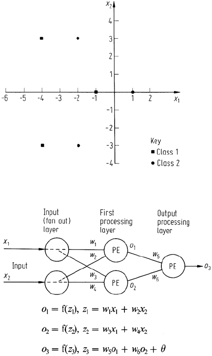
develop the solution to a classiﬁcation problem. Figure 8.21 shows two classes of

data, with three points in each, arranged so that they cannot be separated linearly. The

network shown in Fig. 8.22 will be used to discriminate the data. The two PEs in the

ﬁrst processing layer are described by activation functions with no thresholds – i.e.

θ = 0 in (8.37), while the single output PE has a non-zero threshold in its activation

function.

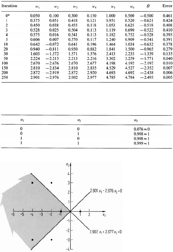
Table 8.3 shows the results of training the network with the backpropagation

method of the previous sections, along with the error measure of (8.40) at each

step. It can be seen that the network approaches a solution quickly (approximately

50 iterations) but takes more iterations (approximately 250) to converge to a ﬁnal

result.

8.9 Non-parametric Classiﬁcation: Geometric Approaches 239

Fig. 8.21. Two-class data set, which is

not linearly separable

Fig. 8.22. Two processing

layer neural network to

be applied to the data of

Fig. 8.21

Having trained the network it is now possible to understand how it implements a

solution to the nonlinear pattern recognition problem. The arguments of the activation

functions of the PEs in the ﬁrst processing layer each deﬁne a straight line (hyperplane

in general) in the pattern space. Using the result at 250 iterations, these are:

2.901x

− 2.976x

= 0

2.902x

+ 2.977x

= 0

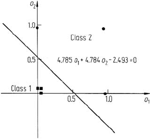
which are shown plotted in Fig. 8.23. An individual line goes some way towards

separating the data but cannot accomplish the task fully. It is now important to

consider how the output PE operates on the outputs of the ﬁrst layer PEs to complete

the discrimination of the two classes. For pattern points lying exactly on one of the

above lines, the output of the respective PE will be 0.5, given that the activation

function of (8.38) has been used. However, for patterns a little distance away from

240 8 Supervised Classiﬁcation Techniques

Table 8.3. Training the network of Fig. 8.22

* arbitrary initial set of weights and θ

Table 8.4. Response of the output layer PE

Fig. 8.23. Neural network solution for the data of Fig. 8.21

8.9 Non-parametric Classiﬁcation: Geometric Approaches 241

Fig. 8.24. Illustration of how the ﬁrst process-

ing layer PEs transform the input data into a

linearly separable set, which is then discrimi-

nated by the output layer hyperplane

those lines the output of the ﬁrst layer PEs will be close to 0 or 1 depending on

which side of the hyperplane they lie. We can therefore regard the pattern space as

being divided into two regions–0and1–byaparticular hyperplane. Using these

extreme values, Table 8.4 shows the possible responses of the output layer PE for

patterns lying somewhere in the pattern space. As seen, for this example the output

PE functions in the nature of a logical OR operation; patterns that lie on the 1 side

of EITHER input PE hyperplane are labelled as belonging to one class, while those

that lie on the 0 side of both hyperplanes will be labelled as belonging to the other

class. Thus patterns which lie in the shaded region shown in Fig. 8.23 will generate a

0 at the output of the network and thus will be labelled as belonging to class 1, while

patterns in the unshaded regions will generate a 1 response and thus will be labelled

as belonging to class 2. Although this exercise is based only on two classes of data,

similar functionality of the various PEs in a network can, in principle, be identiﬁed.

The input PEs will always set up hyperplane divisions of the data and the later PEs

will operate on the results of those simple discriminations.

An alternative way of considering how the network determines a solution is to

regard the ﬁrst processing layer PEs as transforming the data in such a way that

later PEs (in this example only one) can exercise linear discrimination. Figure 8.24

shows a plot of the outputs of the ﬁrst layer PEs when fed with the training data

of Fig. 8.21. As observed, after transformation, the data is linearly separable. The

hyperplane shown is that generated by the argument of the activation function of the

output layer PE.

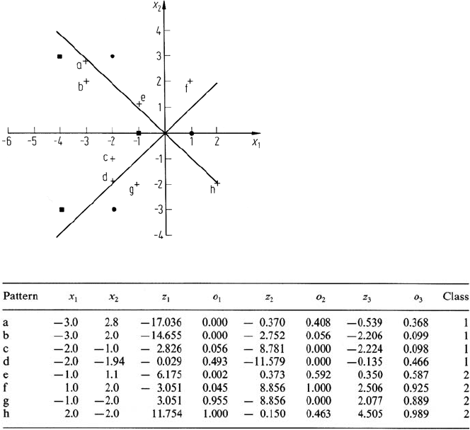
To illustrate how the network of Fig. 8.22 functions on unseen (i.e. testing set)

data, Table 8.5 shows its response to the testing patterns indicated in Fig. 8.25. The

class decision for a pattern is made by rounding the output PE response to 0 or 1 as

appropriate. As noted, for this simple example, all patterns are correctly classiﬁed.

Benediktsson, Swain and Esroy (1990) have demonstrated the application of a

neural network approach to classiﬁcation in remote sensing, obtaining classiﬁcation

accuracies as high as 95% on training data although only as high as 52% when the

network was applied to a test data set. It is suggested that the training data may not

have been fully representative of the image. This is an important issue with neural

242 8 Supervised Classiﬁcation Techniques

Fig. 8.25. Location of test data, indi-

cated by the lettered crosses

Table 8.5. Performance of the network on the test data

nets, more so than with statistical classiﬁcation methods such as maximum likeli-

hood, since the parameters in the statistical approach are estimates of statistics, and

are not strongly affected by outlying training samples. The work of Benediktsson also

illustrates, to an extent, the dependence of performance on the network architecture

chosen.

Hepner (1990) has also used a neural network to perform a classiﬁcation; in

addition to the spectral properties of a pixel, however, he included the spectral mea-

surements of the 3 ×3 neighbourhood in order to allow spatial context to inﬂuence

the labelling. Although quantitative accuracies are not given, Hepner is of the view

that the results are better than when using a maximum likelihood classiﬁer trained

on spectral data only. Lippmann (1987) and Pao (1989) are good general references

to consult for a wider treatment of neural network theory than has been given here,

including other training methods. Both demonstrate also how neural networks can be

used in unsupervised as well as supervised classiﬁcation. Paola and Schowengerdt

(1995a,b) provide a comprehensive review of the use of the multilayer Perception in

remote sensing.

A range of neural network tools is available in MATLAB (1984–2004).