Pump Handbook by Igor J. Karassik, Joseph P. Messina, Paul Cooper, Charles C. Heald - 3rd edition
Подождите немного. Документ загружается.


Jet Pumps
C•H•A•P•T•E•R•4

SECTION 4.1
JET PUMP THEORY
RICHARD G. CUNNINGHAM
4.3
INTRODUCTION______________________________________________________
The jet pump transfers energy from a liquid or gas primary fluid to a secondary fluid.
The latter may be a liquid, a gas, a two-phase gas-in-liquid mixture, or solid particles
transported in a gas or a liquid. Examples of all these combinations have been reported
in the technical literature. Reference 1, the major bibliography in this field, contains
over 400 abstracts.Although the terms “ejector” and “eductor” are also applied, the term
“jet pump” will be used here. The jet pump offers significant advantages over mechani-
cal pumps: no moving parts for improved reliability, adaptability to installation in
remote or hazardous environments, simplicity, and low cost. The primary drawback is
efficiency: both frictional losses and unavoidable mixing losses are incurred. Neverthe-
less, careful design can produce pumps with efficiencies on the order of 30
—
40%. The jet
pump in Figure 1 is typical of liquid-jet pumps and low Mach-number gas-jet/gas pumps.
Compressible-flow pumps, for example, steam-jet ejectors, employ converging-diverging
nozzles for full expansion of the jet.
NOMENCLATURE ____________________________________________________
A area, ft
2
(m
2
)
A
w
throat wall area, ft
2
(m
2
)
C velocity of sound, ft/sec (m/s)
CR cavitation resistance
D diameter, ft (m)
4.4 CHAPTER FOUR
E energy rate, ft lb/sec (joule/s)
K friction loss coefficient
°K absolute temperature, Kelvin
LJL liquid-jet liquid pump
LJG liquid-jet gas compressor
LJGL liquid-jet gas and liquid pump
M liquid/liquid flow ratio, Q
2
/Q
1
MN Mach number
N pressure ratio, LJL jet pump
NPSH net positive suction head
P, P pressure: static, total psia (kPa abs.)
P
v
vapor pressure, psia (kPa abs.)
Q volumetric rate, ft
3
/sec (m
3
/s)
R gas constant, ft lbs/slug °R (joules/kg °K)
°R absolute temperature, Rankine
S density ratio, r
2
/r
1
T temperature °R (°K)
V velocity, ft/sec (m/sec)
W work rate, ft lbs/sec (joules/s)
Z jet dynamic pressure, psi (kPa)
a diffuser area ratio, A
i
/A
d
b jet pump area ratio, A
n
/A
t
c A
2G0
/A
n
(A
t
A
n
)/A
n
(1 b)/b
m mass flow rate, slugs/s (kg/s)
s seconds
psi pounds per square inch
psia pounds per square inch, absolute
r
v
gas/liquid vol. flow rate ratio Q
G
/Q
2
r
v0
gas/liquid vol. flow rate ratio at 0: Q
G0
/Q
2
r
m
gas/liquid mass flow-rate ratio
sp nozzle-to-throat spacing, ft(m)
sp/D
th
spacing, throat diameters
h efficiency
g gas density ratio at s, r
Gs
/r
1
gf
s
m
Gs
/m
1
r density, slugs/ft
3
(kg/m
3
)
t shear stress, psi (kPa)
f gas flow ratio Q
G
/Q
1
f
s
gas flow ratio Q
Gs
/Q
1
at s
Subscripts
1 liquid primary flow
2 liquid secondary flow
4.1 JET PUMP THEORY 4.5
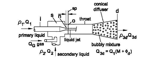
FIGURE 1 Liquid-jet gas and liquid pump and nomenclature
G gas secondary flow
2G bubbly secondary flow
2G0 bubbly sec. flow at 0
mep maximum efficiency point
op operating point
L limit for cavitating flow
3 combined fluids 1, 2, and G
i, s, n locations (see Fig. 1)
0, t, d locations (see Fig. 1)
c0 flow-ratio cut off
f friction loss
n nozzle
en throat entry
th mixing throat
di diffuser
td throat and diffuser
Subscript Examples
Q
2
secondary liquid vol. flow rate
Q
G0
secondary gas flow rate, at 0
Q
2G0
flow rate of bubbly mixture of gas in the secondary liquid, at 0
NOTE:
The convention for pressure and stress in this section is to use psi (and psia) for
pounds per square inch (and pounds per square inch absolute) instead of the conventional
lb/in
2
used throughout the rest of the handbook.
LIQUID-JET PUMP THEORY FOR THREE SECONDARY-FLOW TYPES _________
The liquid-jet pump model is based on conservation equations for energy, momentum, and
mass. Real-fluid losses are accounted for by friction-loss coefficients (K). The primary or
motive fluid is a liquid of density r
1
. In the following derivation, the secondary/pumped fluid

4.6 CHAPTER FOUR
can be a second liquid of density r
1
or r
2
, or a gas-in-liquid bubbly mixture, or a gas. These
three jet pump flow regimes are referred to as liquid-jet liquid (LJL), liquid-jet gas liquid
(LJGL), and liquid-jet gas (LJG). Equations (1), (3), (5), and (7) below apply to all three.
Assumptions:
a. The primary and secondary streams enter the mixing throat with uniform velocity
distributions, and the mixed flows leave the throat and diffuser with a uniform
velocity profile.
b. The gas phase
—
if present
—
undergoes isothermal compression in the throat and diffuser.
c. All two-phase flows at the throat entry and exit consist of homogeneous bubble mix-
tures of a gas in a continuous liquid.
d. Heat transfer from the gas to the liquid is negligible
—
the liquid temperature remains
constant.
e. Change in solubility of the gas in the liquid from pressure P
s
to P
d
is negligible.
f. Vapor evolution from and condensation to the liquid are negligibly small.
NOZZLE EQUATION With reference to Figure 1
(1)
For
the nozzle equation is
THROAT-ENTRY EQUATION The two-phase secondary flow is described by
(2)
Density of the secondary fluid as a function of static pressure and flow ratios M and f is
Integration of Eq. (2) using this density relation and continuity results in the throat-entry
equation:
(3)
MIXING THROAT MOMENTUM EQUATION Equating control volume forces and fluid momentum
changes:
M1P
s
P
o
2 P
s
f
s
ln
P
s
P
o
Z
SM gf
s
c
2
11 K
en
21M f
o
2
2
r
2G
m
2
m
G
Q
2
Q
G
m
1
c
m
2
m
1
m
G
m
1
d
Q
1
1M f2
r
1
c
SM gf
s
m f
d
dP
r
VdV d aK
en
V
2
2
b 0
P
i
P
O
Z11 K
n
2
P
i
P
i
P
i
r
1
V
i
2
2
P
o
r
1
V
2
n
2
K
n
r
1
V
2
n
2
4.1 JET PUMP THEORY 4.7
(4)
where
Substituting the density and continuity relations in Eq. (4) and diving A
th
produces a qua-
dratic equation in P
t
. The throat momentum equation becomes
(5)
DIFFUSER EQUATION The mixed primary and secondary fluids flow from t to d:
The t-d flow is described by Eq. (6):
(6)
Integrating Eq. (6) and substituting the density and continuity relations, the diffuser
equation becomes
(7)
LIQUID-JET PUMP EQUATIONS The liquid jet pump is described in terms of the four flow
processes by Equations (1), (3), (5), and (7). The term gf
s
r
Gs
Q
Gs
/r
1
Q
1
. For isothermal
flow, gf
s
144P
s
f
s
/RT
s
r
1
. For air, with R 1716 ft lb/slug °R, and water, r
1
1.94 slugs/ft
3
and gf
s
.0432P
s
f
s
/T
s
. In SI, R 286.92 mN/kg °K, r
1
1000 kg/m
3
, and gf
s
.00348P
s
f
s
/T
s
, with P
s
in kN/m2, and T
s
in °K. The R and/or r
1
values must of course be
replaced for fluids other than water and air.
In the LJGL pump, the secondary flow is a bubbly mixture of a gas in a liquid. Com-
pressible flow phenomena must be considered because the velocity of sound is quite low in
bubbly fluids. For example, the velocity of sound in a 50/50 uniform mixture of air in water
is about 70 ft/s (21.3 m/s), far below sonic velocities in air (1100 ft/s or 335 m/s) or water
(5000 ft/s or 1524 m/s).
311 M f
t
2
2
a
2
11 M f
d
2
2
K
di
11 M f
t
211 M24
1P
d
P
t
2
P
s
f
s
1 M
ln
P
d
P
t
Zb
2
c
1 SM gf
s
1 M
d
d
t
dP
r
d
t
VdV
d
t
¢P
f
r
3t
0
V
3t
R
3t
V
3d
R
3d
t
d
Z3b
2
12 K
th
211 SM gf
s
2P
s
f
s
4 0
21SM gf
s
21M f
0
2
b
2
11 b2
P
0
Z
dP
t
P
t
2
Z c2b b
2
12 K
th
211 SM gf
s
211 M2
tA
w
A
th
K
th
r
3t
V
2
3t
2
1P
0
P
t
2
A
th
tA
w
1m
1
m
2
m
G
2 V
3t
m
1
V
n
1m
2
m
G
2 V
2G0
V
2Go
V
3t
R
2Go,
R
1,
V
n
R
3t
t
T
o
4.8 CHAPTER FOUR
The Mach number of a bubbly secondary flow at the throat entrance is (see Reference 5):
(8)
When this Mach number is 1.0, the LJGL pump has reached limiting flow; that is, a reduc-
tion in back pressure P
d
no longer causes an increase in the bubbly secondary-flow rate.
Pump Efficiencies The LJGL pump produces two useful work results:
• Static-pressure increase of the liquid component of the secondary flow stream.
• If a gas is entrained in this liquid stream, isothermal compression of the gas component.
With W as the work rate, ft-lb/s, (power) W
L
Q
2
(P
d
P
s
) is the work rate on the liquid
component, and W
G
r
Gs
Q
Gs
RTln(P
d
P
s
) is the work rate on the gas component. The
energy rate input is E
in
Q
1
(P
i
P
s
). The LJGL pump mechanical efficiency is the total
work rate divided by the energy rate in
(9)
The Jet Loss Jet pumps in practical applications have nozzle-to-throat spacings sp/Dth
of one or more mixing-throat diameters. The power jet traverses from a static pressure
at or near P
s
down to P
o
, with no useful work recognized in the one-dimensional theory.
Thus a “jet loss” occurs, which is in addition to the frictional and mixing losses (see Ref-
erence 9).
In the LJL and LJGL (but not the LJG) pumps, throat-inlet pressure drops
—
and hence
jet losses
—
are significant (Ref. 6).
Pump Efficiency, Incorporating Jet Loss In Eq. (9), (P
i
P
d
) is expanded: (P
i
P
d
)
(P
i
P
s
) (P
d
P
s
), and (P
i
P
s
) (P
i
P
o
) (P
s
P
o
) Z(1 K
n
) j(P
s
P
o
),
where j 1 for a fully inserted nozzle, no jet loss: and j 0 for the usual case of retracted
nozzle, which produces full jet loss. Eq. 9 now becomes
(10)
Eq. (10) is recommended for predicting liquid-jet pump efficiencies as follows: Use j
0 for pumps with normally-retracted nozzles (full jet loss); use j 1 for no-jet-loss pumps
(thin-walled nozzle tip fully inserted so sp 0). The pressure in Eq. (10) should be calcu-
lated from the one-dimensional theory using Eqs (1), (3), (5), and (7). (See below for the
LJL jet pump.)
Computer Programs for LJGL and LJG Models Solutions for the compressible flow
cases are generated using computer spreadsheet or Fortran programs. Values for Z, b, P
s
,
Ts, R, r
1
, S and the four K coefficients are fixed/assumed for each pump and operating
conditions. Eqs. (3), (5), and (7) are then solved for each step increase in flow-ratio M, with
f
s
held constant. Alternatively, M may be held constant and the equations solved for step
increase in f
s
. Eqs. (3), (5), and (7) are interdependent: solution of Eq. (5) requires P
o
val-
ues from Eq. (3) and solution of Eq. (7) requires P
t
values from Eq. (5). The program out-
puts at each flow-ratio step are static pressure P
o
, P
t
P
d
, and the three pump efficiencies
defined by Eq. 10.
LJGL FLOW CUT-OFF Compressible-flow choking of the secondary stream at the throat
entrance will occur at MN
o
1. The flow ratio at which this will occur can be predicted
from critical-flow theory. For further details, see Reference 5.
h
M1P
d
P
s
2 P
s
f
s
ln
P
d
P
s
Z11 K
n
2 j1P
s
P
o
2 1P
d
P
s
2
h
L
h
G
h
M1P
d
P
s
2 P
s
f
s
ln
P
d
P
s
P
i
P
d
h
L
h
G
MN
2G0
V
2G0
C
2G0
f
0
c A
2Z
P
s
f
s
1SM gf
s
2
4.1 JET PUMP THEORY 4.9
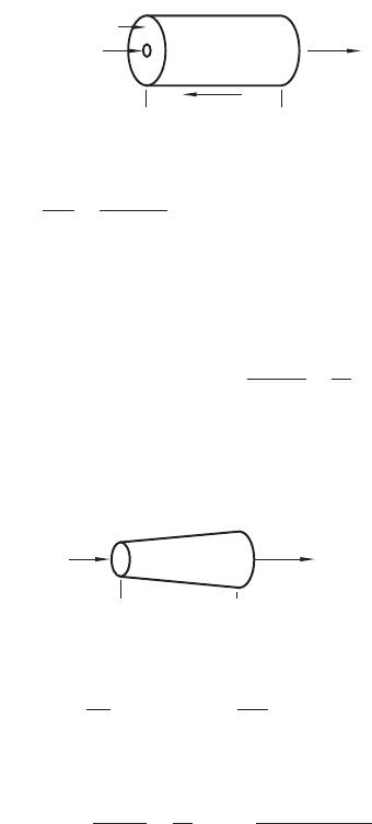
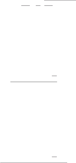
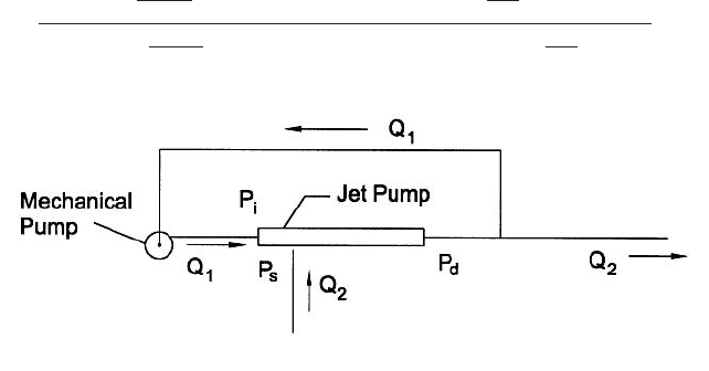
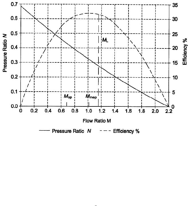
FIGURE 2 LJL jet pump and installation
Performance of the gas compressor (LJG) can be calculated from Eqs. (1), (3), (5), and
(7) by setting M 0. Although simplified, the equations are still coupled as in the LJGL
case. The one-dimensional theory predicts actual performance quite well (see References
6 and 7) provided the mixing is completed within the length of the mixing throat. Theory-
experiment agreement fails and the gas compressor efficiency declines
—
mixing is allowed
to extend into the diffuser.
THE LIQUID-JET LIQUID (LJL) PUMP ____________________________________
Equations for the LJL pump are much simpler than the corresponding LJGL and LJG
equations because of the elimination of all f terms. In this case, Eqs. (1), (3), (5), and (7)
reduce to the following set:
Nozzle (1)
Throat Entry (11)
Throat (12)
Diffuser (13)
Pump efficiency h is defined as the ratio of useful work rate on the secondary fluid Q
2
to
the energy extracted from the primary liquid:
(14)
Two other definitions of efficiency are found in the literature, as follows:
These two other definitions assume that the primary/power stream pressure falls to P
s
, not
P
d
, as shown in Figure 2. Efficiency conversions are possible only if all three pressures and
two flow rates involved are given. Comparisons of efficiencies reported in the literature
should be made with caution.
Combining Eqs. 1, 11
—
14, the theoretical pressure characteristic N for the LJL pump is
(15)
N
2b
2SM
2
b
2
1 b
b
2
11 K
td
a
2
211 M211 SM2 a
SM
2
c
2
b11 K
en
2
1 K
n
2b
2SM
2
b
2
1 b
b
2
11 K
td
a
2
211 M211 SM2 11 j2a
SM
2
c
2
b11 K
en
2
h'' 1M 121P
d
P
s
2> 1P
i
P
s
2
h' Q
2
1P
d
P
s
2>Q
1
1P
i
P
s
2 h>N 1
h Q
2
1P
d
P
s
2>Q
1
1P
i
P
d
2 MN
P
d
P
t
Z
b
2
11 SM211 M211 K
di
a
2
2
P
t
Po Z32b 2SM
2
b
2
>11 b2 b
2
12 K
th
211 SM211 M24
P
s
P
o
ZS11 K
en
2M
2
>c
2
P
i
P
o
Z11 K
n
2
4.10 CHAPTER FOUR
TABLE 1 Performance versus M, for b .25, K
n
.05, K
td
.2, K
en
0
M (P
d
P
s
)/Z (P
i
P
d
)/ZN h%
0.000 0.4250 0.6250 0.6800 0.00
0.200 0.3942 0.6558 0.6012 12.02
0.400 0.3619 0.6881 0.5259 21.04
0.600 0.3280 0.7220 0.4543 27.26
0.800 0.2926 0.7574 0.3862 30.90
1.000 0.2556 0.7944 0.3217 32.17
1.200 0.2170 0.8330 0.2605 31.26
1.400 0.1769 0.8731 0.2026 28.36
1.600 0.1352 0.9148 0.1478 23.65
1.800 0.0920 0.9580 0.0960 17.29
2.000 0.0472 1.0028 0.0471 9.42
2.200 0.0009 1.0491 0.0008 0.19
2.204 0.0000 1.0500 0.0000 0.00
0.676 0.3147 0.7353 0.4280 28.93
1.014 0.2529 0.7971 0.3173 32.17
where K
td
K
th
K
di
. The term j 0 for the normal (jet loss) case, and J 1 for no jet loss.
Jet pumps normally are designed with a finite nozzle-throat spacing, typically sp/D
th
1;
jet loss is experienced, and thus j 0 for this (usual) case. Eq. (15) becomes
(16)
In terms of pressure,
Two simplifications of Eq. (16) are often appropriate: 1) The area ratio term a
2
0 for the
usual 5°
—
8° included-angle diffuser (a A
t
/A
d
is small). 2) The density ratio S 1 for sim-
ilar primary and secondary liquids, for example, a water primary jet pumping water as the
secondary fluid. With these simplifications, Eq. (16) for the normal (jet loss) case becomes
(17)
And pump efficiency is
(18)
For the LJL jet pump, note also that
(19)
Computer Programs for LJL Models It is convenient to use Eqs. (17) and (18) in
spreadsheet form to generate tables of “N(b, M, K
n
, K
td
, K
en
);” that is, the LJL jet pump
pressure characteristic N as a function of the bracketed variables. Typically the Ks and
the area ratio b are held constant and a table is generated using step increases in M to
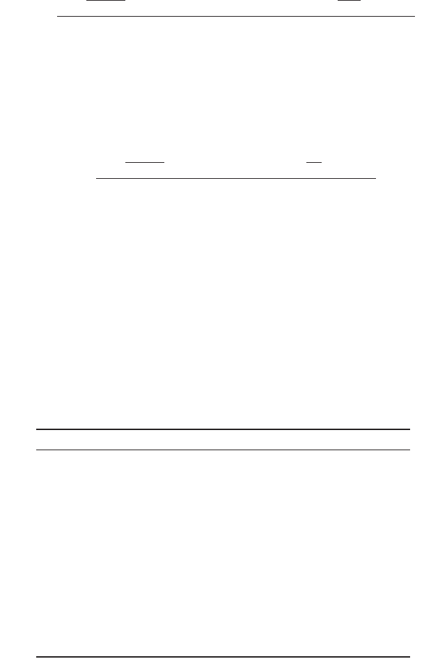
show resultant N values. Table 1 shows N(M) for b .25; and K
n
.05, K
td
.2, and K
en
0. The performance of this pump is shown in Figure 3 as N(M) and h(M).
1P
d
P
s
2> 1P
i
P
s
2 N>1N 12
h h
L
MN
N
2b
2SM
2
b
2
1 b
b
2
11 K
td
211 M2
2
a
M
2
c
2
b11 K
en
2
1 K
n
numerator
N 1P
d
P
s
2> 1P
i
P
d
2
N
2b
2SM
2
b
2
1 b
b
2
11 K
td
a
2
211 M211 SM2 a
SM
2
c
2
b11 K
en
2
1 K
n
numerator
4.1 JET PUMP THEORY 4.11
FIGURE 3 K
n
.05, K
td
.20, K
en
0
It has been shown (see References 2, 3, 4) that one-dimensional analyses successfully
predict actual LJL pump performance. But theory-experiment agreement obtains only if
the test-pump flow conforms with the model assumptions. Two conditions that will cause
departure of measured N and h data from the theoretical curves are
• Cavitation, which occurs in the mixing throat
• Extension of the throat mixing process out into the diffuser
Operating Flow Ratio M
op
In Figure 3, the flow ratio M
op
is indicated on the left slope
of the “parabolic” efficiency curve, which peaks at M M
mep
. The recommended location
of the design operating point is to set M
op
M
mep
. Higher operating M ratios would pro-
vide slightly higher efficiencies, but at a greater risk of cavitation. (Cavitation as part of
the design process is included in the following examples given.) Finding M
mep
can be read-
ily accomplished from Table 1 type data using spreadsheet successive approximations.
Alternatively, Eqs. (17)
—
(18) can be differentiated and set equal to zero to find the peak
efficiency M
mep
value.
Cavitation LJL pumps may encounter cavitation, which occurs in the mixing throat.
With reference to Figure 3, the LJL pump normally responds to a reduction in back pres-
sure P
d
(Q
1
and P
s
constant) by producing a larger Q
2
secondary flow, and hence a larger
M. Measured pressure ratios (N) and efficiencies (h) track along these theory-based char-
acteristic curves as shown in Figure 3. But after the throat-inlet pressure (P
o
) is reduced
to the vapor pressure (P
v
) of the secondary liquid, any further drop in the back pressure
has no effect on the flow ratio, which stabilizes at M M
L
, the cavitation-limited flow
ratio. Note the vertical dashed line in Figure 3: measured N and h values fall on this ver-
tical line, under M
L
operating conditions. In this manner, cavitating-pump performance
departs radically from predicted/normal behavior.
Published studies (see References 1 and 8) have shown that NPSH-type correlations
adequately explain and predict cavitation-limited flow phenomena. Comparing the pre-
dicted M
L
with the intended M
op
is an essential step in designing a jet pump
2
3