Principles of Finance with Excel (Основы финансов c Excel)

Подождите немного. Документ загружается.

PFE, Chapter 13: The CAPM and SML page 20

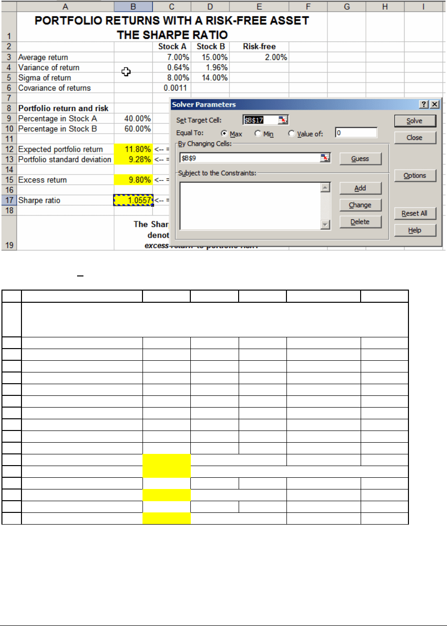
Pressing

Solve yields the answer:

ABCDEF

Stock A Stock B Risk-free

Average return 7.00% 15.00% 2.00%

Variance of return 0.64% 1.96%

Sigma of return 8.00% 14.00%

Covariance of returns 0.0011

Portfolio return and risk

Percentage in Stock A 51.81%

Percentage in Stock B 48.19%

Expected portfolio return 10.85% <-- =B9*C3+B10*D3

Portfolio standard deviation 8.26% <-- =SQRT(B9^2*C4+B10^2*D4+2*B9*B10*C6)

Excess return 8.85% <-- =B12-E3

Sharpe ratio 1.0716 <-- =(B12-E3)/B13

PORTFOLIO RETURNS WITH A RISK-FREE ASSET

THE SHARPE RATIO

From now on, we’ll denote the portfolio with the maximum Sharpe ratio by M:

PFE, Chapter 13: The CAPM and SML page 21

Given a risk-free asset and a set of risky assets (in the current example there are

only 2 such assets), the market portfolio M is the portfolio that maximizes the

Sharpe ratio:

()

−

is larger for M than for any other portfolio.

The portfolio M is the best combination of risky assets available to the

investor.

13.4. The security market line (SML): A remarkable fact

We now show a remarkable fact about expected returns. This fact, called the security

market line

(SML) states that the expected return of an asset or portfolio is determined by the

asset’s risk (called

), the risk-free rate, and the portfolio which maximizes the Sharpe ratio.

Summing up the SML first (then we’ll explain)

The SML says that the expected return on any portfolio of assets is related to the risk-

free rate and the market risk-premium through the following relation

()

(

)

()

is the return

on the portfolio which

maximizes the Sharpe

ratio

pf Mf

Cov r r

Er r Er r

Var r



=+ −



↑↑

Note that in the above equation “portfolio” (represented by the letter “p”) can be a lot of things:

PFE, Chapter 13: The CAPM and SML page 22

• A “portfolio” can be the combination of two risky assets—60% in Stock A and 40% in

Stock B.

•

A “portfolio” can be just one risky asset—100% of your wealth invested in Stock A is a

portfolio.

•

A “portfolio” can be a combination of the risk-free asset and the two stocks—25% in the

risk-free, 30% in Stock A, and 45% in Stock B is a portfolio.

In short: The SML defines the risk-return relation for all assets in the market. In the

next 2 chapters we examine the uses of

for evaluating the performance of portfolio managers

and for computing the cost of capital for a firm.

In order to illustrate the SML, we use a few examples.

Example 1: The SML works for a portfolio composed only of stock A

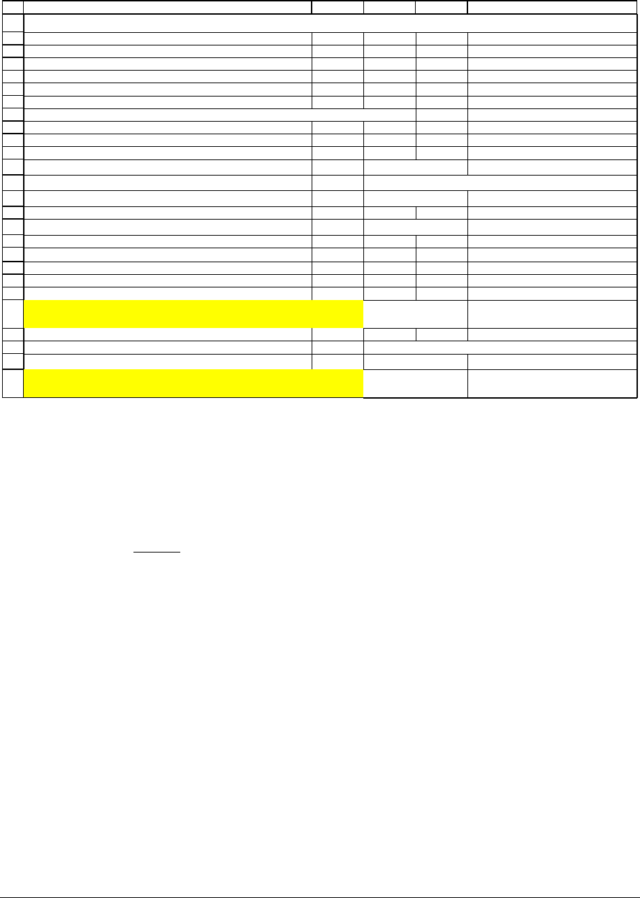
Lines 3-15 of the spreadsheet below repeat facts we’ve already given. In row 24 we

compute the covariance between a portfolio p and the market portfolio M. If p is composed of a

combination of stock A and stock B, then this covariance is given by:

()

(

)

()

()()() ()

,*1,*1

** , 1 *1 * ,

*1 , 1 * * ,

pM A B A B

ABB

AB BA

Cov r r Cov x r x r y r y r

yCovrr x y Covrr

yCovr r x y Covr r

=+−+−

=+−−

+− +−

Cell B24 computes this for our portfolio p (in this case, p is composed wholly of asset A). In cell

B25 we divide Cov(r

) by Var(r

) to get the beta of the portfolio,

PFE, Chapter 13: The CAPM and SML page 23

ABCDE

Stock

Stock B Risk-free

Average return 7.00% 15.00% 2.00%

Variance of return 0.0064 0.0196

Sigma of return 8.00% 14.00%

Covariance of returns 0.0011

Market portfolio M--this is the portfolio that maximizes the Sharpe ratio

Percentage in Stock A 0.5181

Percentage in Stock B 0.4819

Expected market portfolio return, E(r

)

10.85% <-- =B9*B3+B10*C3

Market portfolio return variance, σ

=Var(r

)

0.0068 <-- =B9^2*B4+B10^2*C4+2*B9*B10*B6

Market portfolio standard deviation σ

=standard deviation(r

)

8.26% <-- =SQRT(B13)

Market excess return E(r

)-r

8.85% <-- =B12-D3

"Proof" of SML: E(r

) = r

p*[E(r

) - r

]

Portfolio

Proportion of stock A, x 100.00%

Proportion of stock B, 1-x 0.00%

Expected portfolio return E(r

)=x*E(r

)+(1-x)*E(r

)

SML, left-hand side

7.00% <-- =B20*B3+B21*C3

Cov(portfolio,Market) 0.0039 <-- =B20*B9*B4+B21*B10*C4+B20*B10*B6+B21*B9*B6

Beta β

0.5647 <-- =B24/B13

+β

*[E(r

)-r

]

SML,right-hand side

7.00% <-- =D3+B25*B16

THE SECURITY MARKET LINE (SML)

Now look at the expected portfolio return (7%) given in cell B22 and the expected

portfolio return in cell B26. Though computed in different ways, they’re the same. This is the

SML:

()

pf p Mf

Cov r r

Var r

rr Err

↑



=+ −



Notice that the beta of stock A was computed as

= 0.5647.

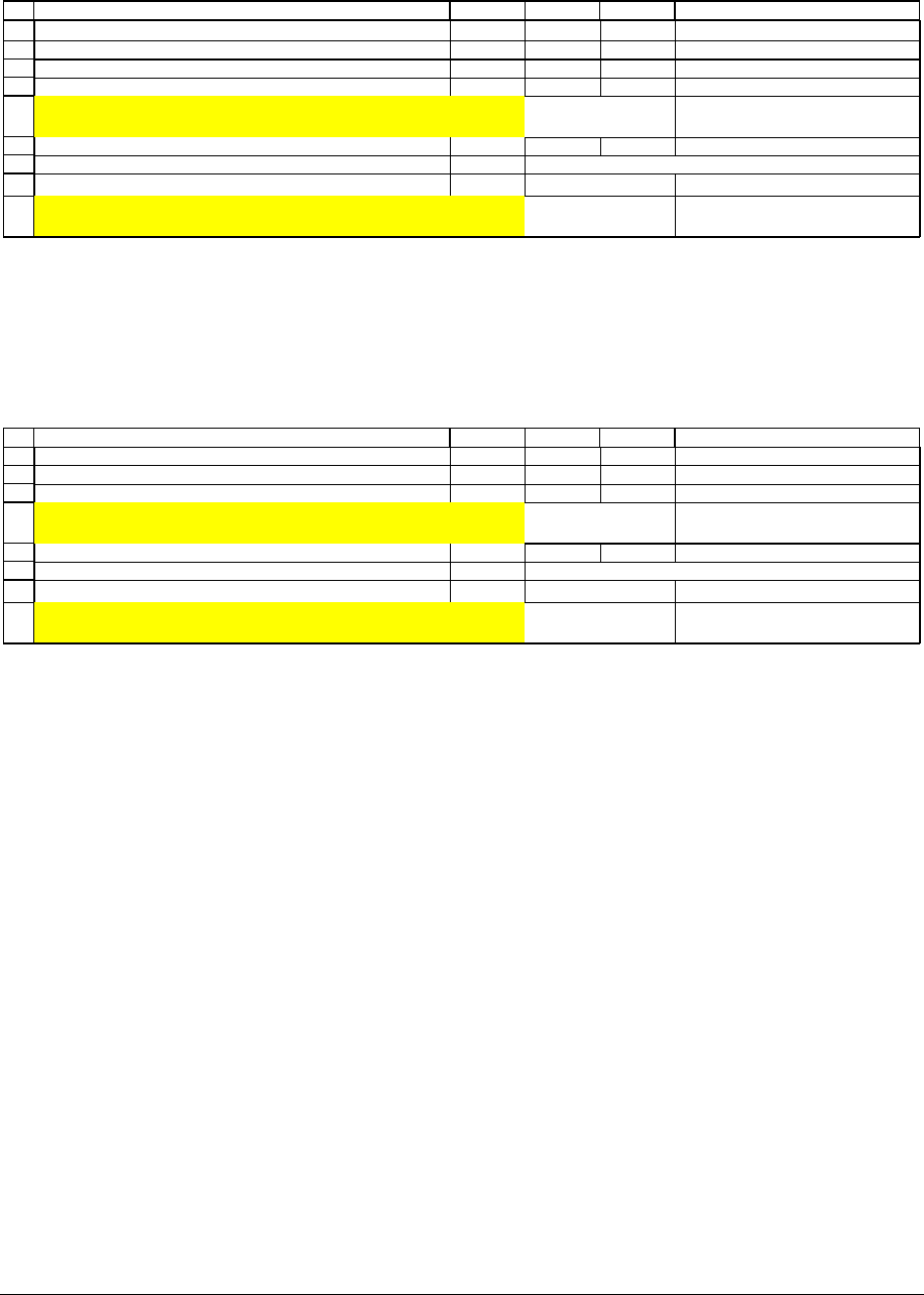
Example 2: The SML works for a portfolio composed only of stock B

Without too much bullshit, we’ll repeat the calculations for stock B. This stock turns out

to have a

= 1.4681:

PFE, Chapter 13: The CAPM and SML page 24

ABCDE

"Proof" of SML: E(r

) = r

p*[E(r

) - r

]

Portfolio

Proportion of stock A, x 0.00%

Proportion of stock B, 1-x 100.00%

Expected portfolio return E(r

)=x*E(r

)+(1-x)*E(r

)

SML, left-hand side

15.00% <-- =B20*B3+B21*C3

Cov(portfolio,Market) 0.0100 <-- =B20*B9*B4+B21*B10*C4+B20*B10*B6+B21*B9*B6

Beta β

1.4681 <-- =B24/B13

+β

*[E(r

)-r

]

SML,right-hand side

15.00% <-- =D3+B25*B16

Again notice that the SML works.

Example 3: The SML works for mixed portfolios

ABCDE

Portfolio

Proportion of stock A, x 80.00%

Proportion of stock B, 1-x 20.00%

Expected portfolio return E(r

)=x*E(r

)+(1-x)*E(r

)

SML, left-hand side

8.60% <-- =B20*B3+B21*C3

Cov(portfolio,Market) 0.0051 <-- =B20*B9*B4+B21*B10*C4+B20*B10*B6+B21*B9*B6

Beta β

0.7453 <-- =B24/B13

+β

*[E(r

)-r

]

SML,right-hand side

8.60% <-- =D3+B25*B16

PFE, Chapter 13: The CAPM and SML page 25

A statistical note (skip this if statistics scares you)

The calculation of

(

)

Cov r r is based on the fact that the covariance is

linear and multiplicative:

(

)

(

)

(

)

() ()

Linear: , , ,

Multiplicative: , ,

Cov x y z Cov x z Cov y z

Cov ax z aCov x z

+= +

Applying this to

()

Cov r r

, gives:

()

()( )

() ()

pp MM

p M GM GM MSFT MSFT GM GM MSFT MSFT

pM pM

GM GM GM GM GM GM MSFT GM

pM pM

SFT MSFT GM GM MSFT MSFT MSFT MSFT

pM pM

GM GM GM GM GM MSFT GM GM

MSFT GM MSFT

Covrr Covxr x r xr x r

Cov x r x r Cov x r x r

Covxr xr Covxr xr

xxCovr r xx Covr r

xxCovr

=+ +

() ( )

() ()

GM MSFT MSFT MSFT MSFT

pM pM

GM GM GM GM MSFT GM GM

pM pM

MSFT GM MSFT GM MSFT MSFT MSFT

rxxCovrr

xxVarr xx Covr r

xxCovr r xxVarr

Betas add up

The portfolio beta is the weighted average of the individual betas:

pGMGMMSFTMSFT

ββ

For example, suppose we want to know the expected return from a portfolio invested

20% in stock A and 80% in stock B. This portfolio will have a

of:

0.2*0.5647 0.8*1.4681 1.0164

pAABB

ββ

=+= + = ,

and consequently its expected return should be determined by the SML using the

PFE, Chapter 13: The CAPM and SML page 26

ABC

0.5647

1.4681

Portfolio composition

Percentage A 50%

Percentage B 50%

Portfolio beta, β

1.0164 <-- =B6*B2+B7*B3

BETAS ADD UP

Summing up

The capital asset pricing model (CAPM) is a model of portfolio formation and asset

pricing. The model shows:

•

How the expected return and standard deviation of portfolios are affected by the portfolio

composition.

•

How the addition of a risk-free asset to the choices available to investors changes their

risk-return opportunity set.

•

How to compute the market portfolio M. This is the portfolio which maximizes the

Sharpe ratio:

(

)

−

•

How to choose an optimal portfolio when you can invest in risky and risk-free assets.

This is the capital market line (CML) which states that all optimal portfolios are

combinations of the risk-free asset and the market portfolio.

PFE, Chapter 13: The CAPM and SML page 27

• How to compute the beta for a stock or portfolio. Beta (

) is a risk-measure for an asset.

For a portfolio p,

is defined as:

(

)

Cov r r

= . (Recall that “portfolio” includes

the case of individual assets.)

•

How the expected return of any portfolio is related to the risk-free rate and the portfolio’s

beta. This is the security market line (SML):

()

(

)

pfp mf

rr Err





=+ −





In succeeding chapters we explore the implications of this model, using it to examine the

performance of portfolio managers and to calculate a firm’s cost of capital.

PFE, Chapter 13: The CAPM and SML page 28

EXERCISES

1. Consider the following portfolio and accompanying statistics:

Company A

Company B

Portfolio Composition

90% 10%

Average Return

21% 48%

Variance

6.15% 16%

Sigma

24.81% 39.40%

Covariance of Returns

0.00390

Correlation of Returns

0.03986

1.a. Is this an optimal portfolio?

1.b. If not, suggest a portfolio combination, which improves return while maintaining the

same level of risk.

1.c. Calculate the minimum variance portfolio for the portfolio composed of the two

assets described above.

2. Using the data provided in the previous question, calculate the market portfolio M, when the

risk-free rate of return is 8%. (Recall that the M portfolio is that portfolio which maximizes the

Sharpe ratio).

3. On the occasion of your birthday, your wealthy Aunt Hilda sends you a check for $5,000,

under the express condition that you invest the money in either (or all) of the following:

Government Bonds, Hilda’s Hybrids Inc., and/or Hilda’s Hubby Inc. The relevant statistics on

each of these investments are provided below.

PFE, Chapter 13: The CAPM and SML page 29

Hilda's Hybrids

Hilda's Hubby Government Bond

Average Return

30.00% 16.25% 10.00%

Variance

28.58% 2.30% 0.00%

Sigma

53.46% 15.17% 0.00%

Covariance of Returns

0.03425

Correlation of Returns

0.42240

3.a. Show the Capital Market Line, i.e. all the combinations of investment in the risk-free

asset and the two companies. Provide results in both chart and graph form. Note that it

will be helpful to first calculate the market portfolio M.

3.b. Supposing you decided to invest in the following proportions, 40% government

bonds, 60% in the M portfolio. Calculate the expected return and variance of returns for

this portfolio.

4. With reference to Question 3 above, you are feeling lucky and decide to take on a riskier

portfolio. In particular, in addition to your $5,000 gift, you are able to borrow another $1,000 at

the risk-free rate of 10%. You decide to invest this total of $6,000 in a portfolio containing a mix

of Hilda’s Hybrids and Hilda’s Hubby.

4.a. In what proportion will you invest your $6,000, if your objective is to create the

“best combination” of these risky assets?

4.b. What will be the expected return and the expected risk for this more daring

portfolio?

5. a. Consider the data below. Compute the expected return and standard deviation of returns

for a portfolio composed of 75% stock A and 25% stock B.