Patrick F. Dunn, Measurement, Data Analysis, and Sensor Fundamentals for Engineering and Science, 2nd Edition

Подождите немного. Документ загружается.

16 Measurement and Data Analysis for Engineering and Science

2.1 Chapter Overview

We live in a world full of electronic devices. Stop for a minute and think of

all the ones you encounter each day. The clock radio usually is the ﬁrst. This

electronic marvel contains a digital display, a microprocessor, an AM/FM

radio, and even a piezoelectric buzzer whose annoying sound beckons us

to get out of bed. Before we even leave for work we have used electric

lights, shavers, toothbrushes, blow dryers, coﬀee pots, toasters, microwave

ovens, refrigerators, and televisions, to name a few. At the heart of all these

devices are electrical circuits. For us to become competent experimentalists,

we need to understand the basics of the electrical circuits present in most

instruments. In this chapter we will review some of the basics of electrical

circuits. Then we will examine several more detailed circuits that comprise

some common measurement systems.

2.2 Concepts and Deﬁnitions

Before proceeding to examine the basic electronics behind a measurement

system’s components, a brief review of some fundamentals is in order. This

review includes the deﬁnitions of the more common quantities involved in

electrical circuits, such as electric charge, electric current, electric ﬁeld, elec-

tric potential, resistance, capacitance, and inductance. The SI dimensions

and units for electric and magnetic systems are summarized in tables on

the text web site. The origins of these and many other quantities involved

in electromagnetism date back to a period rich in the ascent of science, the

17th through mid-19th centuries.

2.2.1 Charge

Electric charge, q, previously called electrical vertue [1], has the SI unit of

coulomb (C) named after the French scientist Charles Coulomb (1736-1806).

The eﬀect of charge was observed in early years when two similar materials

were rubbed together and then found to repel each other. Conversely, when

two dissimilar materials were rubbed together, they became attracted to

each other. Amber, for example, when rubbed, would attract small pieces

of feathers or straw. In fact, electron is the Greek word for amber.

It was Benjamin Franklin (1706-1790) who argued that there was only

one form of electricity and coined the relative terms positive and negative

charge. He stated that charge is neither created nor destroyed, rather it is

conserved, and that it only is transferred between objects. Prior to Franklin’s

Electronics 17

declarations, two forms of electricity were thought to exist: vitreous, from

glass or crystal, and resinous, from rubbing material like amber [1]. It now is

known that positive charge indicates a deﬁciency of electrons and negative

charge indicates an excess of electrons. Charge is not produced by objects,

rather it is transferred between objects.

2.2.2 Current

The amount of charge that moves per unit time through or between materi-

als is electric current, I. This has the SI unit of an ampere (A), named after

the French scientist Andre Ampere (1775-1836). An ampere is a coulomb

per second. This can be written as

I = dq/dt. (2.1)

Current is a measure of the ﬂow of electrons, where the charge of one elec-

tron is 1.602 177 33 × 10

−19

C. Materials that have many free electrons

are called conductors (previously known as non-electrics because they eas-

ily would lose their charge[1]). Those with no free electrons are known as

insulators or dielectrics (previously known as electrics because they could

remain charged) [1]. In between these two extremes lie the semi-conductors,

which have only a few free electrons. By convention, current is considered to

ﬂow from the anode (the positively charged terminal that loses electrons)

to the cathode (the negatively charged terminal that gains electrons) even

though the actual electron ﬂow is in the opposite direction. Current ﬂow

from anode to cathode often is referred to as conventional current. This

convention originated in the early 1800’s when it was assumed that posi-

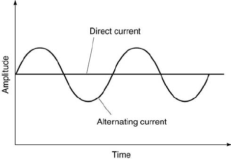
tive charge ﬂowed in a wire. Direct current (DC) is constant in time and

alternating current (AC) varies cyclically in time, as depicted in Figure

2.1. When current is alternating, the electrons do not ﬂow in one direction

through a circuit, but rather back and forth in both directions. The symbol

for a current source in an electrical circuit is given in Figure 2.2.

2.2.3 Force

When electrically charged bodies attract or repel each other, they do so

because there is an electric force acting between the charges on the bodies.

Coulomb’s law relates the charges of the two bodies, q

and q

, and the

distance between them, R, to the electric force, F

, by the relation

= Kq

, (2.2)

where K = 1/(4π

), with the permittivity of free space 

= 8.854 187 817

× 10

−12

F/m. The SI unit of force is the newton (N).

18 Measurement and Data Analysis for Engineering and Science

FIGURE 2.1

Direct and alternating currents.

2.2.4 Field

The electric ﬁeld, E, is deﬁned as the electric force acting on a positive

charge divided by the magnitude of the charge. Hence, the electric ﬁeld has

the SI unit of newtons per coulomb. This leads to an equivalent expression

= qE. So, the work required to move a charge of 1 C a distance of 1 m

through a unit electric ﬁeld of 1 N/C is 1 N·m or 1 J. The SI unit of work

is the joule (J).

2.2.5 Potential

The electric potential, Φ, is the electric ﬁeld potential energy per unit

charge, which is the energy required to bring a charge from inﬁnity to an

arbitrary reference point in space. Often it is better to refer to the poten-

tial diﬀerence, ∆Φ, between two electric potentials. It follows that the SI

unit for electric potential is joules per coulomb. This is known as the volt

(V), named after Alessandro Volta (1745-1827). Volta invented the voltaic

pile, originally made of pairs of copper and zinc plates separated by wet

paper, which was the world’s ﬁrst battery. In electrical circuits, a battery is

indicated by a longer, solid line (the anode) separated over a small distance

by a shorter, solid line (the cathode), as shown in Figure 2.3. The symbol

for a voltage source is presented in Figure 2.2.

2.2.6 Resistance and Resistivity

When a voltage is applied across the ends of a conductor, the amount of

current passing through it is linearly proportional to the applied voltage.

Electronics 19

FIGURE 2.2

Basic circuit element symbols.

The constant of proportionality is the electric resistance, R. The SI unit

of resistance is the ohm (Ω), named after Georg Ohm (1787-1854).

Electric resistance can be related to electric resistivity, ρ, for a wire of

cross-sectional area A and length L as

R = ρL/A. (2.3)

The SI unit of resistivity is Ω·m. Conductors have low resistivity values

(for example, Ag: 1.5 × 10

−8

Ω·m), insulators have high resistivity values

(for example, quartz: 5 × 10

Ω·m), and semi-conductors have intermediate

resistivity values (for example, Si: 2 Ω·m).

Resistivity is a property of a material and is related to the temperature

of the material by the relation

ρ = ρ

[1 + α(T − T

)], (2.4)

20 Measurement and Data Analysis for Engineering and Science

FIGURE 2.3

The battery.

where ρ

denotes the reference resistivity at reference temperature T

and

α the coeﬃcient of thermal expansion of the material. For conductors, α

ranges from approximately 0.002/

◦

C to 0.007/

◦

C. Thus, for a wire

R = R

[1 + α(T − T

)]. (2.5)

2.2.7 Power

Electric power is electric energy transferred per unit time, P (t) =

I(t)V (t). Using Ohm’s law, it can be written also as P (t) = I

(t)R. This

implies that the SI unit for electric power is J/s or watt (W).

2.2.8 Capacitance

When a voltage is applied across two conducting plates separated by an

insulated gap, a charge will accumulate on each plate. One plate becomes

charged positively (+q) and the other charged equally and negatively (−q).

The amount of charge acquired is linearly proportional to the applied volt-

age. The constant of proportionality is the capacitance, C. Thus, q = CV .

The SI unit of capacitance is coulombs per volt (C/V). The symbol for

capacitance, C, should not be confused with the unit of coulomb, C. The

SI unit of capacitance is the farad (F), named after the British scientist

Michael Faraday (1791-1867).

2.2.9 Inductance

When a wire is wound as coil and current is passed through it by applying

a voltage, a magnetic ﬁeld is generated that surrounds the coil. As the

current changes in time, a changing magnetic ﬂux is produced inside the coil,

which in turn induces a back electromotive force (emf). This back emf

opposes the original current, leading to either an increase or a decrease in the

current, depending upon the direction of the original current. The resulting

magnetic ﬂux, φ, is linearly proportional to the current. The constant of

proportionality is called the electric inductance, denoted by L. The SI

unit of inductance is the henry (H), named after the American Joseph Henry

(1797-1878). One henry equals one weber per ampere.

Electronics 21

Element

Unit Symbol

I(t)

V (t)

I=const

Resistor

V (t)/R

RI(t)

Capacitor

CdV (t)/dt

(1/C)

I(τ )dτ

It/C

Inductor

(1/L)

V (τ)dτ

LdI/dt

TABLE 2.1

Resistor, capacitor, and inductor current and voltage relations.

Example Problem 2.1

Statement: 0.3 A of current passes through an electrical wire when the voltage

diﬀerence between its ends is 0.6 V. Determine [a] the wire resistance, R, [b] the total

amount of charge that moves through the wire in 2 minutes, q

total

, and [c] the electric

power, P.

Solution: [a] Application of Ohm’s law gives R = 0.6 V/0.3 A = 2 Ω. [b] Integration

of Equation 2.1 gives q(t) =

I(t)dt. Because I(t) is constant, q

total

= (0.3 A)(120

s) = 36 C. [c] The power is the product of current and voltage. So, P = (0.3 A)(0.6 V)

= 0.18 W = 0.2 W, with the correct number of signiﬁcant ﬁgures.

2.3 Circuit Elements

At the heart of all electrical circuits are some basic circuit elements. These

include the resistor, capacitor, inductor, transistor, ideal voltage source, and

ideal current source. The symbols for these elements that are used in circuit

diagrams are presented in Figure 2.2. These elements form the basis for

more complicated devices such as operational ampliﬁers, sample-and-hold

circuits, and analog-to-digital conversion boards, to name only a few (see

[2]).

The resistor, capacitor, and inductor are linear devices because the

complex amplitude of their output waveform is linearly proportional to the

amplitude of their input waveform. A device is linear if [1] the response to

(t) + x

(t) is y

(t) + y

(t) and [2] the response to ax

(t) is ay

(t), where

a is any complex constant [4]. Thus, if the input waveform of a circuit com-

prised only of linear devices, known as a linear circuit, is a sine wave of

a given frequency, its output will be a sine wave of the same frequency.

Usually, however, its output amplitude will be diﬀerent from its input am-

plitude and its output waveform will lag the input waveform in time. If the

lag is between one-half to one cycle, the output waveform appears to lead

the input waveform, although it always lags the input waveform. The re-

22 Measurement and Data Analysis for Engineering and Science

sponse behavior of linear systems to various input waveforms is presented

in Chapter 4. The current-voltage relations for the resistor, capacitor, and

inductor are summarized in Table 2.1.

2.3.1 Resistor

The basic circuit element used more than any others is the resistor. Its

current-voltage relation is deﬁned through Ohm’s law,

R = V/I. (2.6)

Thus, the current in a resistor is related linearly to the voltage diﬀerence

across it, or vice versa. The resistor is made out of a conducting material,

such as carbon, carbon-ﬁlm, or metal-ﬁlm. Typical resistances range from a

few ohms to more than 10

Ω.

2.3.2 Capacitor

The current ﬂowing through a capacitor is related to the product of its

capacitance and the time rate of change of the voltage diﬀerence, where

I =

= C

. (2.7)

For example, 1 µA of current ﬂowing through a 1 µF capacitor signiﬁes that

the voltage diﬀerence across the capacitor is changing at a rate of 1 V/s. If

the voltage is not changing in time, there is no current ﬂowing through the

capacitor. The capacitor is used in circuits where the voltage varies in time.

In a DC circuit, a capacitor acts as an open circuit. Typical capacitances

are in the µF to pF range.

2.3.3 Inductor

Faraday’s law of induction states that the change in an inductor’s magnetic

ﬂux, φ, with respect to time equals the applied voltage, dφ/dt = V (t).

Because φ = LI,

V (t) = L

. (2.8)

Thus, the voltage across an inductor is related linearly to the product of its

inductance and the time rate of change of the current. The inductor is used

in circuits in which the current varies in time. The simplest inductor is a wire

wound in the form of a coil around a nonconducting core. Most inductors

have negligible resistance when measured directly. When used in an AC

circuit, the inductor’s back emf controls the current. Larger inductances

impede the current ﬂow more. This implies that an inductor in an AC circuit

acts like a resistor. In a DC circuit, an inductor acts as a short circuit.

Typical inductances are in the mH to µH range.

Electronics 23

2.3.4 Transistor

The transistor was developed in 1948 by William Shockley, John Bardeen,

and Walter Brattain at Bell Telephone Laboratories. The common transis-

tor consists of two types of semiconductor materials, n-type and p-type. The

n-type semiconductor material has an excess of free electrons and the p-type

material a deﬁciency. By using only two materials to form a pn junction,

one can construct a device that allows current to ﬂow in only one direc-

tion. This can be used as a rectiﬁer to change alternating current to direct

current. Simple junction transistors are basically three sections of semicon-

ductor material sandwiched together, forming either pnp or npn transistors.

Each section has its own wire lead. The center section is called the base,

one end section the emitter, and the other the collector. In a pnp tran-

sistor, current ﬂow is into the emitter. In an npn transistor, current ﬂow

is out of the emitter. In both cases, the emitter-base junction is said to be

forward-biased or conducting (current ﬂows forward from p to n). The op-

posite is true for the collector-base junction. It is always reverse-biased or

non-conducting. Thus, for a pnp transistor, the emitter would be connected

to the positive terminal of a voltage source and the collector to the nega-

tive terminal through a resistor. The base would also be connected to the

negative terminal through another resistor. In such a conﬁguration, current

would ﬂow into the emitter and out of both the base and the collector. The

voltage diﬀerence between the emitter and the collector causing this cur-

rent ﬂow is termed the base bias voltage. The ratio of the collector-to-base

current is the (current) gain of the transistor. Typical gains are up to ap-

proximately 200. The characteristic curves of a transistor display collector

current versus the base bias voltage for various base currents. Using these

curves, the gain of the transistor can be determined for various operating

conditions. Thus, transistors can serve many diﬀerent functions in an elec-

trical circuit, such as current ampliﬁcation, voltage ampliﬁcation, detection,

and switching.

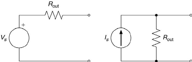
FIGURE 2.4

Voltage and current sources.

24 Measurement and Data Analysis for Engineering and Science

2.3.5 Voltage Source

An ideal voltage source, shown in Figure 2.4, with R

out

= 0, maintains a

ﬁxed voltage diﬀerence between its terminals, independent of the resistance

of the load connected to it. It has a zero output impedance and can supply

inﬁnite current. An actual voltage source has some internal resistance. So

the voltage supplied by it is limited and equal to the product of the source’s

current and its internal resistance, as dictated by Ohm’s law. A good voltage

source has a very low output impedance, typically less than 1 Ω. If the

voltage source is a battery, it has a ﬁnite lifetime of current supply, as

speciﬁed by its capacity. Capacity is expressed in units of current times

lifetime (which equals its total charge). For example, a 1200 mA hour battery

pack is capable of supplying 1200 mA of current for 1 hour or 200 mA for 6

hours. This corresponds to a total charge of 4320 C (0.2 A × 21 600 s).

2.3.6 Current Source

An ideal current source, depicted in Figure 2.4, with R

out

= ∞ maintains

a ﬁxed current between its terminals, independent of the resistance of the

load connected to it. It has an inﬁnite output impedance and can supply

inﬁnite voltage. An actual current source has an internal resistance less than

inﬁnite. So the current supplied by it is limited and equal to the ratio of the

source’s voltage diﬀerence to its internal resistance. A good current source

has a very high output impedance, typically greater than 1 MΩ. Actual

voltage and current sources diﬀer from their ideal counterparts only in that

the actual impedances are neither zero nor inﬁnite, but ﬁnite.

2.4 RLC Combinations

Linear circuits typically involve resistors, capacitors, and inductors con-

nected in various series and parallel combinations. Using the current-

voltage relations of the circuit elements and examining the potential dif-

ference between two points on a circuit, some simple rules for various com-

binations of resistors, capacitors, and inductors can be developed.

First, examine Figure 2.5 in which the series combinations of two resis-

tors, two capacitors, and two inductors are shown. The potential diﬀerence

across an i-th resistor is IR

, across an i-th capacitor is q/C

, and across

an i-th inductor is L

dI/dt. Likewise, the total potential diﬀerence, V

, for

the series resistors’ combination is V

= IR

, for the series capacitors’

combination is V

= q/C

, and for the series inductors’ combination is

= L

dI/dt. Because the potential diﬀerences across resistors, capaci-

tors, and inductors in series add, V

= V

+ V

. Hence, for the resistors’

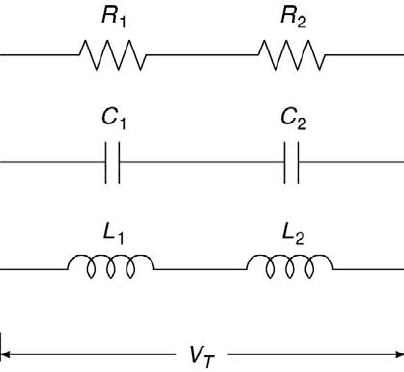
Electronics 25

FIGURE 2.5

Series R, C, and L circuit conﬁgurations.

series combination, V

= IR

+ IR

= IR

, which yields

= R

+ R

. (2.9)

For the capacitors’ series combination, V

= q/C

+ q/C

= q/C

, which

implies

1/C

= 1/C

+ 1/C

. (2.10)

For the inductors’ series combination, V

= L

dI/dt + L

dI/dt = L

dI/dt,

which gives

= L

+ L

. (2.11)

Thus, when in series, resistances and inductances add, and the reciprocals

of capacitances add.

Next, view Figure 2.6 in which the parallel combinations of two resistors,

two capacitors, and two inductors are displayed. The same expressions for

the i-th and total potential diﬀerences hold as before. Hence, for the resistors’

parallel combination, I

= I

+ I

, which leads to

1/R

= 1/R

+ 1/R

. (2.12)

For the capacitors’ parallel combination, q

= q

+ q

, which leads to

= C

+ C

. (2.13)

For the inductors’ parallel combination, I

= I

+ I

, which gives

1/L

= 1/L

+ 1/L

. (2.14)