Pao Y.C. Engineering Analysis: Interactive Methods and Programs with FORTRAN, QuickBASIC, MATLAB, and Mathematica

Подождите немного. Документ загружается.

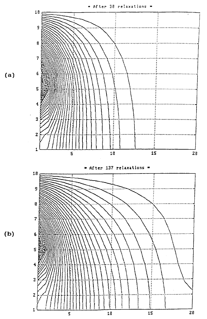
FIGURE 5. After 38 relaxations (a) and after 137 relaxations (b).

along the upper edge (Y = 10) and right edge (X = 20), the ﬁrst curved contour of

the right has a value equal to 1, and the values of the contours are increased from

right to left until the point marked “5” which has a temperature equal to 50 is

reached. It should be noted that along the left edge, the uppermost point marked

“10” has a temperature equal to zero and the temperatures are increased linearly (as

for the initial conditions) to 50 at the point marked with “5”, and from that point

down to the point marked “1” the entire lower portion of the left edge is insulated.

For obtaining the 137th sweep, we can continue to call the service Relaxatn.m

by similarly applying the MATLAB instructions as follows:

>> for NR = 31:137; [D,T] = feval(A:Relaxatn',T]; end

>> fprintf('Sweep # %3.0f \n',NR),D,T

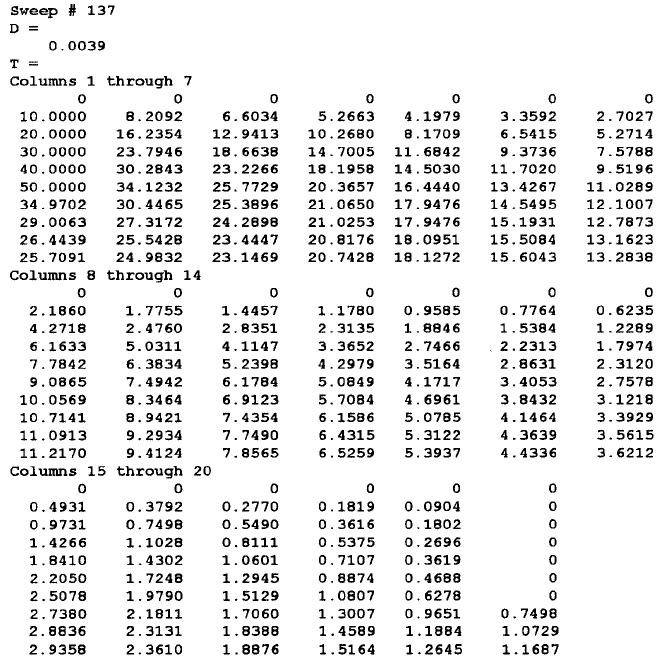
The resulting display of the error deﬁned in Equation 13 and the 137th temper-

ature distribution is:

Figure 5b shows the 137th temperature distribution when the interactive MAT-

LAB instructions entered are:

>> V = 0:1:50; contour(T,V’), grid, title(‘* After 137 relaxations *’)

Notice that area near the insulated boundaries at the right-lower corner has ﬁnally

reached a steady-state temperature distribution, i.e., changes of the entire temperature

distribution will be insigniﬁcant if more relaxations were pursued.

MATHEMATICA APPLICATIONS

To apply the relaxation method for ﬁnding the steady-state temperature distri-

bution of the heated plate already solved by the FORTRAN, QuickBASIC, and

MATLAB versions, here we make use of the Do, If, and While commands of

Mathematica to generate similar results through the following interactive opera-

tions:

In[1]: = t = Table[0,{10},{20}]; eps = 100; nr = 0; d = eps + 1;

In[2]: = Do[t[[i,1]] = (I–1)*10,{i,2,6}];

In[3]: = (While[d>eps, d = 0;nr = nr + 1;

Do[Do[ts = t[[i,j]]; t[[i,j]] = .25*(t[[I–1,j]] + t[[I + 1,j]]

+ t[[i,j–1]] + t[[i,j + 1]]);

d = Abs[ts-t[[i,j]]] + d;,{j,2,19}],{i,2,6}];

Do[ts = t[[i,1]]; t[[i,1]] = .25*(t[[I–1,1]] + t[[I + 1,1]]

+ 2*t[[i,2]]); d = Abs[ts-t[[i,1]]] + d;

Do[ts = t[[i,j]]; t[[i,j]] = .25*(t[[I–1,j]] + t[[I + 1,j]]

+ t[[i,j–1]] + t[[i,j + 1]]);

d = Abs[ts-t[[i,j]]] + d;,{j,2,19}];

If[i = = 7,Continue, ts = t[[i,20]];

t[[i,20]] = .25*(t[[I–1,20]] + t[[I + 1,20]] + 2*t[[i,19]]);

d = Abs[ts-t[[i,20]]] + d;],{i,7,9}];

ts = t[[10,1]]; t[[10,1]] = .5*(t[[9,1]] + t[[10,2]]);

d = Abs[ts-t[[10,1]]] + d;

Do[ts = t[[10,j]]; t[[10,j]] = .25*(2*t[[9,j]] + t[[10,j–1]]

+ t[[10,j + 1]]); d = Abs[ts-t[[10,j]]] + d;,{j,2,19}];

ts = t[[10,20]]; t[[10,20]] = .5*(t[[9,20]] + t[[10,19]]);

d = Abs[ts-t[[10,20]]] + d;])

In[4]: = Print[“Sweep #”,nr]; Round[N[t,2]]

Out[4] = Sweep #2

{{ 0, 0, 0, 0, 0, 0, 0, 0, 0, 0, 0, 0, 0, 0, 0, 0, 0, 0, 0, 0},

{10, 4, 1, 0, 0, 0, 0, 0, 0, 0, 0, 0, 0, 0, 0, 0, 0, 0, 0, 0},

{20, 9, 3, 1, 0, 0, 0, 0, 0, 0, 0, 0, 0, 0, 0, 0, 0, 0, 0, 0},

{30, 13, 5, 2, 1, 0, 0, 0, 0, 0, 0, 0, 0, 0, 0, 0, 0, 0, 0, 0},

{40, 18, 7, 3, 1, 0, 0, 0, 0, 0, 0, 0, 0, 0, 0, 0, 0, 0, 0, 0},

{50, 20, 8, 3, 1, 0, 0, 0, 0, 0, 0, 0, 0, 0, 0, 0, 0, 0, 0, 0},

{17, 11, 5, 2, 1, 0, 0, 0, 0, 0, 0, 0, 0, 0, 0, 0, 0, 0, 0, 0},

{ 6, 5, 3, 1, 1, 0, 0, 0, 0, 0, 0, 0, 0, 0, 0, 0, 0, 0, 0, 0},

{ 2, 2, 1, 1, 0, 0, 0, 0, 0, 0, 0, 0, 0, 0, 0, 0, 0, 0, 0, 0},

{ 1, 1, 1, 1, 0, 0, 0, 0, 0, 0, 0, 0, 0, 0, 0, 0, 0, 0, 0, 0}}

Notice that In[2] initializes the boundary temperatures, nr keeps the count of

how many sweeps have been performed, and the function Round is employed in

In[4] to round the temperature value to a two-digit integer. When the total temper-

ature differences, d, is limited to eps = 100 degrees, the t values obtained after two

sweeps are slightly different from those obtained by the other versions, this is again

because Mathematica keeps more signiﬁcant digits in all computation steps than

those in the FORTRAN, QuickBASIC, and MATLAB programs. By changing the

eps value from 100 degrees to 1 degree, Mathematica also takes 137 sweeps to

converge as in the FORTRAN, QuickBASIC, and MATLAB versions:

In[5]: = t = Table[0,{10},{20}]; eps = 1; nr = 0; d = eps + 1;

In[6]: = Do[t[[i,1]] = (I–1)*10,{i,2,6}];

In[7]: = Print[“Sweep #”,nr]; Round[N[t,2]]

Out[7] = Sweep #137

{{ 0, 0, 0, 0, 0, 0, 0, 0, 0, 0, 0, 0, 0, 0, 0, 0, 0, 0, 0, 0},

{10, 8, 7, 5, 4, 3, 3, 2, 2, 1, 1, 1, 1, 1, 0, 0, 0, 0, 0, 0},

{20, 16, 13, 10, 8, 7, 5, 4, 3, 3, 2, 2, 2, 1, 1, 1, 1, 0, 0, 0},

{30, 24, 19, 15, 12, 9, 8, 6, 5, 4, 3, 3, 2, 2, 1, 1, 1, 1, 0, 0},

{40, 30, 23, 18, 15, 12, 10, 8, 6, 5, 4, 4, 3, 2, 2, 1, 1, 1, 0, 0},

{50, 34, 26, 20, 16, 13, 11, 9, 7, 6, 5, 4, 3, 3, 2, 2, 1, 1, 0, 0},

{35, 30, 25, 21, 17, 15, 12, 10, 8, 7, 6, 5, 4, 3, 3, 2, 2, 1, 1, 0},

{29, 27, 24, 21, 18, 15, 13, 11, 9, 7, 6, 5, 4, 3, 3, 2, 2, 1, 1, 1},

{26, 26, 23, 21, 18, 16, 13, 11, 9, 8, 6, 5, 4, 4, 3, 2, 2, 1, 1, 1},

{26, 25, 23, 21, 18, 16, 13, 11, 9, 8, 7, 5, 4, 4, 3, 2, 2, 2, 1, 1}}

The above results all agree with those obtained earlier.

WARPING ANALYSIS OF A TWISTED BAR WITH NONCIRCULAR CROSS SECTION

As another example of applying the relaxation method for engineering analysis,

consider the case of a long bar of uniform rectangular cross section twisted by the

two equal torques (T) at its ends. The cross section of the twisted bar becomes

warped as shown in Figure 6. If z-axis is assigned to the longitudinal direction of

the bar, to ﬁnd the amount of warping at any point (x,y) of the cross sectioned

surface, denoted as W(x,y), the relaxation method can again be employed because

W(x,y) is governed by the Laplace equation.

Due to anti-symmetry of W(x,y), that

is W(–x,y) = W(x,–y) = –W(x,y), only one-fourth of the cross section needs to be

analyzed. Let us consider a rectangular region 0≤x≤a and 0≤y≤b. It is obvious that

the anti-symmetry leads to the conditions W(x,0) = 0 and W(0,y) = 0 along two of

the four linear boundaries. To derive the boundary conditions along the right side

x = a and the upper side y = b, we have to utilize the relationships between the

warping function W(x,y) and shear stresses 

and 

which are:

(19,20)

where G and  are the shear rigidity and twisting angle of the bar, respectively.

Along the boundaries x = a and y = b, the shear stress should be tangential to the

lateral surface of the twisted bar requires:

(21)

where s is the variable changed along the boundary. Along the upper boundary y =

b, dy/ds = 0 and dx/ds = 1 and along the right boundary x = a, dx/ds = 0 and dy/ds =

1. Consequently, Equation 19 reduces to:

(22,23)

To apply the relaxation method for solving W(x,y) which satisﬁes the Laplace

equation for 0<x<a and 0<y<b and the boundary conditions W(0,y) = W(x,0) = 0

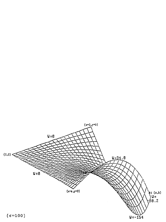
FIGURE 6. In the case of a bar of uniform rectangular cross section twisted by the two

equal torques (T) at its ends, the cross section of the twisted bar becomes warped as shown.

τθ τθ

xz yz

y and G

∂

−













∂













∂

−













−

∂













∂

=− =

∂

x for y b and

y for x a

and Equations 22 and 23, let us partition the rectangular region 0≤x≤a and 0≤y≤b

into a network of MxN using the increments x = a/(M–1) and y = b/(N–1). In

ﬁnite-difference forms, Equations 22 and 23 yield, respectively:

(24)

and

(25)

where x

= (i–1)x and y

= (j–1)y. Equations 24 and 25 can be combined to yield

a ﬁnite-difference formula for relaxing the corner point (x

). That is:

(26)

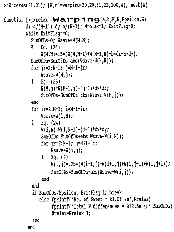
Program Relaxatn.m has been modiﬁed to develop a new m ﬁle Warping.m

for the warping analysis which uses input values for a, b, M, N, and which is needed

in Equation 13 for termination of the relaxation. MATLAB statements for sample

application of Warping.m are listed below along with the m-ﬁle itself. The mesh

plot of the warping surface W(x,y) obtained after 131 sweeps of relaxation by

initially assuming W(x,y) = 0 throughout the entire region and an  value equal to

100 is shown in Figure 7.

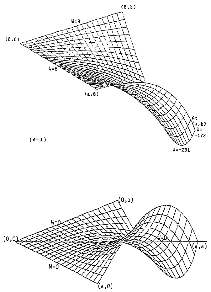
FIGURE 7. The result for  = 100 when a = 30 and b = 20 means that each of the 600

gridpoints is allowed to have, on average, a difference equal to 1/6 during two consecutive

relaxations.

W x y y b W x b y x y for i M

, , , , ,=≡

()

=−

()

−=…−∆∆ 23 1

W x x a y W a x y y x for j N

jjj

=≡

()

=−

()

+=…−, , , , ,∆∆ 23 1

Wx ay b Way Wx b b x a y

MN N M

≡≡

()

+−

[]

−−

,., ,5

∆∆

Notice that the variable Nrelax keeps track how many sweeps have been per-

formed during the relaxation procedure, it is an output argument like W which can

be printed if desired. The exit ﬂag, FlagExit, is initially set equal to zero and changed

to a value of unity when the total error, SumOfDs, is less than and allowing the

relaxation to be terminated.

Figure 7 is the result for  = 100 when a = 30 and b = 20 which means that each

of the 600 gridpoints is allowed to have, on average, a difference equal to 1/6 during

two consecutive relaxations. The W values are found to be in the range of –154 and

24.8 for = 100. When is set equal to 1 which means that each gridpoint is allowed

to have, on the average, a difference of 1/600, the mesh plot of W is shown in

Figure 8. The W values are now all equal to or less than zero.

It is noteworthy that if the cross section of the twisted rod is square, that is when

a = b, there is no warping along the x = y line as illustrated by the mesh plot shown in

Figure 9. This case is left as a homework problem for the readers to work out the details.

FIGURE 8.

FIGURE 9.

8.4 PROGRAM WAVEPDE — NUMERICAL SOLUTION OF WAVE

PROBLEMS GOVERNED BY HYPERBOLIC PARTIAL

DIFFERENTIAL EQUATIONS

Program WavePDE is designed for numerical solution of the wave problems gov-

erned by the hyperbolic partial differential equation.

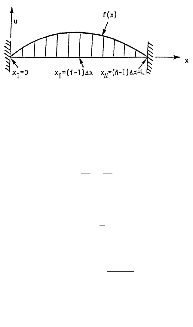
Consider the problem of a

tightened string shown in Figure 10. The lateral displacement u satisﬁes the equation:

(1)

where x is the variable along the longitudinal direction of the string and a is the

wave velocity related to the tension T in the string and the mass m of the string by

the equation:

(2)

Together with the governing equation of u, Equation 1, there are also so-called

initial conditions prescribed which may be expressed as:

(3,4)

f(x) in Equation 3 describe the initial position while v

(x) describes the initial

velocity of the tightened string. And, also there are so-called boundary conditions

which in the case of a string at both ends are:

(5,6)

FIGURE 10. The problem of a tightened string.

∂

u t x f x and

ut x

vx=

()

∂=

()

∂

()

utx x and utx x L

, ,==

()

===

()

00 0

If the string is made of a single material, T/m would then be equal to a constant.

Analytical solution can be found for this simple case. For the general case that the

string may be composed of a number of different materials and the mass m is then

a function of the spatial variable x. The more complicated the variation of these

properties in x and t, the more likely no analytical solution possible and the problem

can only be solved numerically.

The ﬁnite-difference approximation of Equation 1 can be achieved by applying

the central difference for the second derivatives for both with respect to the space

variable x and the time variable t. If we consider the displacement u only a ﬁnite

number of stations, say N, deﬁned with a spatial increment x and using a time

increment of t, then specially, for t at t

and x at x

, we can have:

and

Substituting the above expressions into Equation 1, we obtain:

(7)

Equation 7 is to be applied for j = 2 through j = N–1. Initially for t = t

= 0,

Equation 7 can be applied for i = 2, then u

i–1,j

≡ u(t

) term is simply f(x

) and can

be calculated using Equation 3, and the u

i,j–1

, u

i,j

, and u

i,j + 1

terms can be calculated

using the forward-difference approximations of Equation 4 which are, for k =

2,3,…,N–1

(8)

Since both f(x) and v

(x) are prescribed, use of Equation 7 enables all u to be

calculated at t = t

and at all in-between stations x

, for j = 2,3,…,N–1. When u

values at t = t

and t = t

are completely known, Equation 7 can again be utilized to

compute u at t = t

for i = 4 and so forth. Because the string is tightened, we expect

the magnitudes of u values to continuously decrease in time. That is, for a speciﬁed

tolerance, we may demand that the computation be terminated when

(9)

∂

−−

()

−+

uuu

ij ij ij,, ,

∆

∂

−+

()

−+

uuu

ij ij ij,,,

∆

uuu

i j i j ij ij ij ij+= − +

=− + +









−+

()

,,, ,,,

∆

ut x ut x v x t fx v x t

kkkkk

210 0

()

∆∆

max.

j=2~N-1

ij,

<ε